Understanding Descriptive Statistics in Data Analysis
Descriptive statistics provide a vital framework for analyzing data by focusing on three key characteristics: measures of center, dispersion, and shape. Standard deviation, a fundamental measure, helps assess variability in distributions through the Empirical Rule and Chebyshev's Theorem. These principles aid in interpreting data insights and making informed decisions based on the distribution shape and variability.

Download Presentation

Please find below an Image/Link to download the presentation.
The content on the website is provided AS IS for your information and personal use only. It may not be sold, licensed, or shared on other websites without obtaining consent from the author. Download presentation by click this link. If you encounter any issues during the download, it is possible that the publisher has removed the file from their server.
E N D
Presentation Transcript
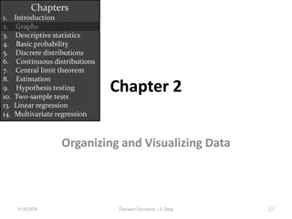
Chapters 1. Introduction 2. Graphs 3. Descriptive statistics 4. Basic probability 5. Discrete distributions 6. Continuous distributions 7. Central limit theorem 8. Estimation 9. Hypothesis testing 10. Two-sample tests 13. Linear regression 14. Multivariate regression Chapter 3 Numerical Descriptive Techniques II
When Describing a Data Set We always report three important characteristics about the data: 1. Measure of center or location 2. Measure of dispersion or spread 3. Measure of shape or symmetry 9/19/2024 Towson University - J. Jung 4.2
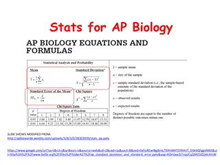
Review: Standard Deviation The standard deviation is simply the square root of the variance, thus: Population standard deviation: Sample standard deviation: 9/19/2024 Towson University - J. Jung 4.3
Interpreting Standard Deviation The standard deviation can be used to compare the variability of several distributions and make a statement about the general shape of a distribution. If the histogram is bell shaped, we can use the Empirical Rule, which states: 1) Approximately 68% of all observations fall within one standard deviation of the mean. 2) Approximately 95% of all observations fall within two standard deviations of the mean. 3) Approximately 99.7% of all observations fall within three standard deviations of the mean. 9/19/2024 Towson University - J. Jung 4.4
The Empirical Rule Approximately 68% of all observations fall within one standard deviation of the mean. Approximately 95% of all observations fall within two standard deviations of the mean. Approximately 99.7% of all observations fall within three standard deviations of the mean. 9/19/2024 Towson University - J. Jung 4.5
ChebysheffsTheorem A more general interpretation of the standard deviation is derived from Chebysheff s Theorem, which applies to all shapes of histograms (not just bell shaped). The proportion of observations in any sample that lie within k standard deviations of the mean is at least: For k=2 (say), the theorem states that at least 3/4 of all observations lie within 2 standard deviations of the mean. This is a lower bound compared to Empirical Rule s approximation (95%). 9/19/2024 Towson University - J. Jung 4.6
Interpreting Standard Deviation Suppose that the mean and standard deviation of last year s midterm test marks are 70 and 5, respectively. If the histogram is bell-shaped then we know that approximately 68% of the marks fell between 65 and 75, approximately 95% of the marks fell between 60 and 80, and approximately 99.7% of the marks fell between 55 and 85. If the histogram is NOT at all bell-shaped we can say that at least 75% of the marks fell between 60 and 80, and at least 88.9% of the marks fell between 55 and 85. (We can use other values of k.) 9/19/2024 Towson University - J. Jung 4.7
Measure of Risk Risk is of key interest in stock market. Standard Deviation or Variance is often used, but is appropriate ONLY when the mean return on investment is the same. When mean return vary greatly, the order of magnitude of the mean influences the size of the variance. Standard Deviation or Variance is not appropriate when comparing dispersion for two items in different units. e.g. How do we compare inches to dollars? 9/19/2024 Towson University - J. Jung 4.8
Coefficient of Variation The coefficient of variation of a set of observations is the standard deviation of the observations divided by their mean, that is: Population coefficient of variation = CV = Sample coefficient of variation = cv = Coefficient of Variation is a better measure, because it Is free of unit measures relative dispersion 9/19/2024 Towson University - J. Jung 4.9
Coefficient of Variation This coefficient provides a proportionate measure of variation, which is free of units It measures relative dispersion. e.g. A standard deviation of 10 may be perceived as large when the mean value is 100, but only moderately large when the mean value is 500. CV is a more reliable measure here. 9/19/2024 Towson University - J. Jung 4.10
Example Returns on stocks: Stock 1: Mean $5 Standard Deviation $10 Stock 2: Mean return: $10,000 Standard Deviation $100 Just looking at standard deviation, you d conclude that there is more variability in stock 2, so that stock 2 is the riskier one. That s not true. The variation in stock 1, adjusted for the mean size of returns is very large compared to the adjusted variation in stock 2. CV1 = 10/5 = 2 -> one s.d. represents a 200% variation in stock return CV2= 100/10,000= 0.01 -> one s.d. represents only 1% variation return 9/19/2024 Towson University - J. Jung 4.11
Measure of Shape How symmetric is the data set? Two equivalent methods. 1 Use measures of center If mean=median=mode, symmetric If mode<median<mean, Right (Positive) Skewed If mean<median<mode, Left (Negative) Skewed 2. Use Pearson s Second Skewness: Sk=0, Symmetric; Sk>0, Right (Positive) Skewed; Sk<0, Left (Negative) Skewed. ( 3 ) Mean Median = Sk ( . ) St Deviation 9/19/2024 Towson University - J. Jung 4.12
Statistics is a pattern language Population Sample N n Size Mean Variance Standard Deviation S s Coefficient of Variation CV= cv= x 9/19/2024 Towson University - J. Jung 4.13
Measures of Variability If data are symmetric, with no serious outliers, use range and standard deviation. If comparing variation across two data sets, use coefficient of variation. The measures of variability introduced in this section can be used only for interval data. 9/19/2024 Towson University - J. Jung 4.14
Measures of Location Provide information about the position of particular values relative to the entire data set. Percentile: the Pth percentile is the value for which P percent are less than that value and (100-P)% are greater than that value. Example: Suppose you scored in the 60th percentile on the GMAT, that means 60% of the other scores were below yours, while 40% of scores were above yours. If your exam mark places you in the 80th percentile, that doesn t mean you scored 80% on the exam it means that 80% of your peers scored lower than you on the exam; its about your position relative to others. 9/19/2024 Towson University - J. Jung 4.15
Quartiles We have special names for the 25th, 50th, and 75th percentiles, namely quartiles. The first or lower quartile is labeled Q1 = 25th percentile. The second quartile, Q2 = 50th percentile (which is also the median). The third or upper quartile, Q3 = 75th percentile. We can also convert percentiles into quintiles (fifths) and deciles (tenths). 9/19/2024 Towson University - J. Jung 4.16
Commonly Used Percentiles First (lower) decile First (lower) quartile, Q1, Second (middle)quartile,Q2, Third quartile, Q3, Ninth (upper) decile = 10th percentile = 25th percentile = 50th percentile = 75th percentile = 90th percentile Note: If your exam mark places you in the 80th percentile, that doesn t mean you scored 80% on the exam it means that 80% of your peers scored lower than you on the exam; It is about your position relative to others. 9/19/2024 Towson University - J. Jung 4.17
Location of Percentiles The following formula allows us to approximate the location of any percentile: 9/19/2024 Towson University - J. Jung 4.18
Location of Percentiles Recall the data from example 4.1: 0 0 5 7 8 9 12 14 22 33 Where is the location of the 25th percentile? That is, at which point are 25% of the values lower and 75% of the values higher? L25 = (10+1)(25/100) = 2.75 0 0 5 7 8 9 12 14 22 33 The 25th percentile is three-quarters of the distance between the second (which is 0) and the third (which is 5) observations. Three-quarters of the distance is: (.75)(5 0) = 3.75 Because the second observation is 0, the 25th percentile is: 0 + 3.75 = 3.75 9/19/2024 Towson University - J. Jung 4.19
Location of Percentiles What about the upper quartile? L75 = (10+1)(75/100) = 8.25 0 0 5 7 8 9 12 14 22 33 It is located one-quarter of the distance between the eighth and the ninth observations, which are 14 and 22, respectively. One-quarter of the distance is: (.25)(22 - 14) = 2, which means the 75th percentile is at: 14 + 2 = 16 9/19/2024 Towson University - J. Jung 4.20
Location of Percentiles Please remember position 2.75 16 0 0 | 5 7 8 9 12 14 | 22 33 position 8.25 3.75 Lp determines the position in the data set where the percentile value is located, not the value of the percentile itself. 9/19/2024 Towson University - J. Jung 4.21
Interquartile Range The quartiles can be used to create another measure of variability, the inter quartile range (IQR), which is defined as follows: Interquartile Range = Q3 Q1 Unlike variance and standard deviation, IQR is insensitive to outliers. The interquartile range measures the spread of the middle 50% of the observations. Large values of this statistic mean that the 1st and 3rd quartiles are far apart indicating a high level of variability. 9/19/2024 Towson University - J. Jung 4.22
Box Plots The box plot is a technique that graphs five statistics: the (1) minimum and (2) maximum observations, and Whisker1: (Q1- 1.5*(Q3 -Q1)) The lines extending to the left and right are called whiskers. Any points that lie outside the whiskers are called outliers. The whiskers extend outward to the smaller of 1.5 times the inter quartile range or to the most extreme point that is not an outlier. Whisker 2: (Q3+ 1.5*(Q3 -Q1)) the (3) first, (4) second, and (5) third quartiles. 9/19/2024 Towson University - J. Jung 4.23
9/19/2024 Towson University - J. Jung 4.24
Example 4.15 A large number of fast-food restaurants with drive-through windows offering drivers and their passengers the advantages of quick service. To measure how good the service is, an organization called QSR planned a study wherein the amount of time taken by a sample of drive- through customers at each of five restaurants was recorded. Compare the five sets of data using a box plot and interpret the results. 9/19/2024 Towson University - J. Jung 4.25
Box Plots Wendy s service time is shortest and least variable. Hardee s has the greatest variability, while Jack-in-the-Box has the longest service times. 9/19/2024 Towson University - J. Jung 4.26
9/19/2024 Towson University - J. Jung 4.27