Network Navigation Models and Local Information

Navigation with
local information
Shai Carmi
Bar-Ilan University
Israel
2009


W
h
y
l
o
c
a
l
i
n
f
o
r
m
a
t
i
o
n
?
The Internet is huge.
So are social networks and
transportation networks.
Navigating with information of the
entire topology is not scalable.
To find target with local information,
we must use heuristics.
* Greedy routing: minimize distance to target.
* Route through nodes of high degree.
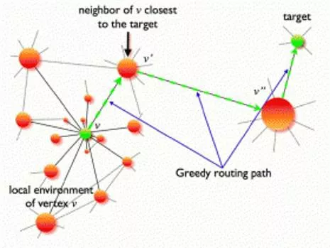
Boguna & Krioukov, PRL 102, 058701 (2009)
Network models- Introduction
In a network, links (edges) connect computers/individuals which are
represented by nodes. There are few network models:
1.
Simplest model: a regular lattice.
* Good for purely spatial, local, interactions.
2.
Erdos-Renyi (ER) network model: fully random.
* Fixed number of nodes
N
, each link exists
with probability
p
.
* Narrow degree distribution:
where
k
is node degree.
3.
Scale-free (SF) networks: emergence of hubs.
* Broad degree distribution:
* Nodes with extremely high degree exist (hubs).
* Other ingredients possible, e.g., growth, correlations.
* Found to describe most real-world systems.
Navigation models: Outline
1.
Searching for the hub.
2.
Kleinberg’s lattice model.
N
a
v
i
g
a
t
i
o
n
m
o
d
e
l
s
1.
Searching for the hub.
2.
Kleinberg’s lattice model.
How to find the most connected node
in the network: An algorithm
Start from a given node.
Go to the neighbor with
highest degree
(break ties arbitrarily).
Keep going, until
reaching a peak-
a node whose degree is
greater than all of its
neighbors.
Basins of attraction
are
formed around each hub.
Only knowledge of the neighbors’ degree is required!
Large-scale example
What is it good for?
A new way of decomposing the network based on the
association to a hub.
In an energy landscape network, can tell us where will
the system end up.
In wireless sensor networks, it is
desirable to deliver a message to
the hub with minimal energy
consumption. If the sensor network
has just one basin, our algorithm
will be useful.
Basins distribution in scale-free networks
How does the basins topology depend on the degree exponent
γ
(
P(k)~k
-
γ
)
?
Q(s)
- the probability of a node to belong
to a basin of size
s
.
We empirically find that
Q(s)~s
-
α
for small
s
.
The size of the largest basin scales
as
S~N
δ
, where
δ
=1
for
γ
≤
γ
c
and
δ
≈1/(
γ
-1)
for large
γ
.
Interpretation: for
γ
≤
γ
c
≈3 a giant basin exists that attracts most nodes.
For large
γ
where the network is more homogeneous it is fragmented to
numerous basins whose size distribution decays as a power-law.
The giant
basin
Theory- a transition at
γ
=3
The probability of a node with degree
k
to be a peak is
approximately exp[-Ak
3-
γ
], where
A
is a
k
-independent constant.
For
γ
<3
, the probability approaches zero-
only the true hub is a peak.
For
γ
>3
, every node with large degree is almost surely a peak.
For large
γ
, the size of the giant basin scales as the size of the
largest degree in the network
S~N
1/(
γ
-1)
.
The first two moments of the
number of basins can be
approximated analytically.
Deterministic fractal
(u,v)
-nets
The behavior Q(s)~s
-
α
can
be explained using a fractal
scale-free network model.
Each link in generation
n
splits into
u+v=w
links in
generation
n+1
.
Generalization to lattices
Instead of degree, node’s importance is determined by a different
attribute such as height or energy.
Assume each node is attracted to its shortest neighbor.
A physical interpretation of the size of the basins of attraction:
place one particle at each node and let the particles follow a path of
steepest descent. The final number of particles in each node is the
size of its basin of attractions.
valley
valley
valley
valley
peak
peak
peak
peak
saddle
saddle
saddle
Results on lattices
Easy to calculate that the number of valleys is
N/3± 2N/45
.
Define
R(s)
as the probability of a node to be a valley of a basin of
size
s
.
In 1D,
R(1)=1/30
, and
R(s)
decays as
1/s!
, much faster than the power-law for networks.
In 2D, the density of peaks and valleys is 1/5, of saddles 1/15.
We find
R(1)=109/4290
. Other values of R are
hard to obtain.
Other features appear such as craters and ridges.
For example, the density of craters is 3/715.
N
a
v
i
g
a
t
i
o
n
m
o
d
e
l
s
1.
Searching for the hub.
2.
Kleinberg’s lattice model.
The navigation problem and Kleinberg’s model
Social networks are small-worlds, meaning that short paths exist.
But how do people find them?
Kleinberg’s model (2000)
* Underlying lattice.
* Nearest neighbors connections.
* One long-range link for each node.
* Probability for a long-range link over
distance
r
decays as
r
--
α
.
*
Greedy routing
: message is always sent
to the neighbor geographically nearest to the destination.
Kleinberg proved (
T- delivery time; d- dimension; L- lattice size
)
In the special case
α
=d
, local
information is enough to find
short paths!
A theory of Kleinberg navigation
Kleinberg only provided lower bounds for
α≠
d
and an upper
bound for
α
=d
but did not find the exact asymptotic behavior.
We write a master equation for T (
using
p
i,i+k
=Ak
-
α
):
We find the
asymptotic solution:
Agrees with
Kleinberg’s bounds.
Simulations
Our solution agrees with
numerical results
(both simulations and
iteration of the master equation).
What happens if messages can be lost?
Define the probability of successful
completion of a single step as
z
.
By modifying the master equation,
we can calculate T
z
(L) analytically.
T
h
e
s
y
s
t
e
m
i
s
s
m
a
l
l
-
w
o
r
l
d
f
o
r
a
m
u
c
h
w
i
d
e
r
r
a
n
g
e
o
f
α
!
E
x
p
l
a
i
n
s
w
h
y
t
h
e
s
y
s
t
e
m
n
e
e
d
n
o
t
b
e
f
i
n
e
-
t
u
n
e
d
t
o
b
e
c
o
m
e
n
a
v
i
g
a
b
l
e
.
No message loss
With message loss
S
u
m
m
a
r
y
Navigation with local information is a problem with interesting practical
and theoretical aspects.
We study, analytically and numerically, the behavior of two models.
Searching for the hub
It is sometimes desirable to find the most
connected node with minimal effort.
Each node is associated with a hub by
walking up the degree gradient.
The network is decomposed into basins
of attractions based on hub association.
A transition in scale-free networks: a
giant basin emerges for
γ
<3
. For
γ
>>3
each high degree node forms a basin.
We derived the basin size distribution for
fractal models and 1D chain.
Kleinberg’s lattice model
Assume individuals are placed on a lattice
with nn links plus one long-range link.
Messages are delivered using knowledge
of neighbors location only.
Only bounds were known for the delivery
time (for 9 years!).
We found exact asymptotic expression for
the delivery time, in agreement with
Kleinberg’s bounds.
Introduction of a fugacity parameter makes
the model more realistic.
Acknowledgements and references
Prof. Daniel ben-Avraham (Clarkson University, NY)
and students Stephen Carter and Jie Sun.
Prof. Paul Krapivsky (Boston University, MA).
My advisor Prof. Shlomo Havlin.
My host in BU Prof. H. Eugene Stanley.
S
h
a
i
C
a
r
m
i
,
P
.
L
.
K
r
a
p
i
v
s
k
y
,
a
n
d
D
a
n
i
e
l
b
e
n
-
A
v
r
a
h
a
m
.
"
P
a
r
t
i
t
i
o
n
o
f
n
e
t
w
o
r
k
s
i
n
t
o
b
a
s
i
n
s
o
f
a
t
t
r
a
c
t
i
o
n
"
.
P
h
y
s
.
R
e
v
.
E
7
8
,
0
6
6
1
1
1
(
2
0
0
8
)
.
S
h
a
i
C
a
r
m
i
,
S
t
e
p
h
e
n
C
a
r
t
e
r
,
J
i
e
S
u
n
,
a
n
d
D
a
n
i
e
l
b
e
n
-
A
v
r
a
h
a
m
.
"
A
s
y
m
p
t
o
t
i
c
b
e
h
a
v
i
o
r
o
f
t
h
e
K
l
e
i
n
b
e
r
g
m
o
d
e
l
"
.
P
h
y
s
.
R
e
v
.
L
e
t
t
.
1
0
2
,
2
3
8
7
0
2
(
2
0
0
9
)
.
Thank you for your attention!
Basins of attraction vs. community detection
The calculation of the basins of attraction provides a decomposition
of the network.
How does it compare with state of the art community detectors?
Most community detectors use global information.
More importantly, community detection and separation to basins
have different goals. Consider this example:
Community detectors:
Maximize links
within communities;
minimize links
between communities.
Basins of attraction:
Separate nodes by
the hub they
associate with.
Not really two communities!
T
i
e
b
r
e
a
k
i
n
g
What happens when the neighbor of highest degree of a node has
the same degree as the node itself?
In our local search, a node can be a peak
even if it has neighbors of equal degree.
In a recursive search, we surf over
“ridges” of connected nodes of equal
degree to reach the true hub.
Less basins exist,
but other results
remain qualitatively
the same.
"In this study, the focus is on network navigation models and the importance of utilizing local information for efficient routing. Different network models and navigation strategies are explored, emphasizing the significance of heuristics and algorithms for finding well-connected nodes in large-scale networks. The discussion covers topics like the emergence of hubs in scale-free networks and the benefits of basins of attraction around highly connected nodes. Practical applications and implications for various network types are also considered."

Download Presentation

Please find below an Image/Link to download the presentation.
The content on the website is provided AS IS for your information and personal use only. It may not be sold, licensed, or shared on other websites without obtaining consent from the author.If you encounter any issues during the download, it is possible that the publisher has removed the file from their server.
You are allowed to download the files provided on this website for personal or commercial use, subject to the condition that they are used lawfully. All files are the property of their respective owners.
The content on the website is provided AS IS for your information and personal use only. It may not be sold, licensed, or shared on other websites without obtaining consent from the author.
E N D
Presentation Transcript
Navigation with local information Shai Carmi Bar-Ilan University Israel 2009
Why local information? The Internet is huge. So are social networks and transportation networks. Navigating with information of the entire topology is not scalable. To find target with local information, we must use heuristics. * Greedy routing: minimize distance to target. * Route through nodes of high degree. Boguna & Krioukov, PRL 102, 058701 (2009)
Network models- Introduction In a network, links (edges) connect computers/individuals which are represented by nodes. There are few network models: 1. Simplest model: a regular lattice. * Good for purely spatial, local, interactions. 2. Erdos-Renyi (ER) network model: fully random. * Fixed number of nodes N, each link exists with probability p. * Narrow degree distribution: where k is node degree. 3. Scale-free (SF) networks: emergence of hubs. * Broad degree distribution: * Nodes with extremely high degree exist (hubs). * Other ingredients possible, e.g., growth, correlations. * Found to describe most real-world systems. k k = ( ) / ! P k e k k k P ) ( k
Navigation models: Outline 1. Searching for the hub. 2. Kleinberg s lattice model.
Navigation models 1. Searching for the hub. 2. Kleinberg s lattice model.
How to find the most connected node in the network: An algorithm Start from a given node. Go to the neighbor with highest degree (break ties arbitrarily). Keep going, until reaching a peak- a node whose degree is greater than all of its neighbors. Basins of attraction are formed around each hub. 3 1 2 2 2 2 1 2 2 4 3 2 3 1 1 1 Only knowledge of the neighbors degree is required!
What is it good for? A new way of decomposing the network based on the association to a hub. In an energy landscape network, can tell us where will the system end up. In wireless sensor networks, it is desirable to deliver a message to the hub with minimal energy consumption. If the sensor network has just one basin, our algorithm will be useful.
Basins distribution in scale-free networks How does the basins topology depend on the degree exponent (P(k)~k- )? The giant basin Q(s)- the probability of a node to belong to a basin of size s. We empirically find that Q(s)~s- for small s. The size of the largest basin scales as S~N , where =1 for c and 1/( -1) for large . Interpretation: for c 3 a giant basin exists that attracts most nodes. For large where the network is more homogeneous it is fragmented to numerous basins whose size distribution decays as a power-law.
Theory- a transition at =3 The probability of a node with degree k to be a peak is approximately exp[-Ak3- ], where A is a k-independent constant. For <3, the probability approaches zero- only the true hub is a peak. For >3, every node with large degree is almost surely a peak. For large , the size of the giant basin scales as the size of the largest degree in the network S~N1/( -1). The first two moments of the number of basins can be approximated analytically.
Deterministic fractal (u,v)-nets The behavior Q(s)~s- can be explained using a fractal scale-free network model. Each link in generation n splits into u+v=w links in generation n+1.
Generalization to lattices Instead of degree, node s importance is determined by a different attribute such as height or energy. Assume each node is attracted to its shortest neighbor. A physical interpretation of the size of the basins of attraction: place one particle at each node and let the particles follow a path of steepest descent. The final number of particles in each node is the size of its basin of attractions. peak valley saddle saddle valley peak peak valley peak saddle valley
Results on lattices Easy to calculate that the number of valleys is N/3 2N/45. Define R(s) as the probability of a node to be a valley of a basin of size s. In 1D, R(1)=1/30, and R(s) decays as 1/s!, much faster than the power-law for networks. In 2D, the density of peaks and valleys is 1/5, of saddles 1/15. We find R(1)=109/4290. Other values of R are hard to obtain. Other features appear such as craters and ridges. For example, the density of craters is 3/715.
Navigation models 1. Searching for the hub. 2. Kleinberg s lattice model.
The navigation problem and Kleinbergs model Social networks are small-worlds, meaning that short paths exist. But how do people find them? Kleinberg s model (2000) * Underlying lattice. * Nearest neighbors connections. * One long-range link for each node. * Probability for a long-range link over distance r decays as r-- . * Greedy routing: message is always sent to the neighbor geographically nearest to the destination. Kleinberg proved (T- delivery time; d- dimension; L- lattice size) In the special case =d, local information is enough to find short paths!
A theory of Kleinberg navigation Kleinberg only provided lower bounds for d and an upper bound for =d but did not find the exact asymptotic behavior. We write a master equation for T (using pi,i+k=Ak- ): We find the asymptotic solution: Agrees with Kleinberg s bounds.
Simulations Our solution agrees with numerical results (both simulations and iteration of the master equation). No message loss What happens if messages can be lost? Define the probability of successful completion of a single step as z. By modifying the master equation, we can calculate Tz(L) analytically. With message loss The system is small-world for a much wider range of ! Explains why the system need not be fine-tuned to become navigable.
Summary Navigation with local information is a problem with interesting practical and theoretical aspects. We study, analytically and numerically, the behavior of two models. Searching for the hub Kleinberg s lattice model It is sometimes desirable to find the most connected node with minimal effort. Each node is associated with a hub by walking up the degree gradient. The network is decomposed into basins of attractions based on hub association. A transition in scale-free networks: a giant basin emerges for <3. For >>3 each high degree node forms a basin. We derived the basin size distribution for fractal models and 1D chain. Assume individuals are placed on a lattice with nn links plus one long-range link. Messages are delivered using knowledge of neighbors location only. Only bounds were known for the delivery time (for 9 years!). We found exact asymptotic expression for the delivery time, in agreement with Kleinberg s bounds. Introduction of a fugacity parameter makes the model more realistic.
Acknowledgements and references Prof. Daniel ben-Avraham (Clarkson University, NY) and students Stephen Carter and Jie Sun. Prof. Paul Krapivsky (Boston University, MA). My advisor Prof. Shlomo Havlin. My host in BU Prof. H. Eugene Stanley. Shai Carmi, P.L. Krapivsky, and Daniel ben-Avraham. "Partition of networks into basins of attraction". Phys. Rev. E 78, 066111 (2008). Shai Carmi, Stephen Carter, Jie Sun, and Daniel ben-Avraham. "Asymptotic behavior of the Kleinberg model". Phys. Rev. Lett. 102, 238702 (2009).
Basins of attraction vs. community detection The calculation of the basins of attraction provides a decomposition of the network. How does it compare with state of the art community detectors? Most community detectors use global information. More importantly, community detection and separation to basins have different goals. Consider this example: Community detectors: Maximize links within communities; minimize links between communities. Basins of attraction: Separate nodes by the hub they associate with. Not really two communities!
Tie breaking What happens when the neighbor of highest degree of a node has the same degree as the node itself? In our local search, a node can be a peak even if it has neighbors of equal degree. 1 1 1 2 2 2 2 3 In a recursive search, we surf over ridges of connected nodes of equal degree to reach the true hub. 1 1 1 2 2 2 2 3 Less basins exist, but other results remain qualitatively the same.


-nets")