Hydrologic Modeling Methods in HEC-HMS: A Comprehensive Overview
Explore the transformative methods within HEC-HMS hydrologic modeling, including unit hydrograph derivation, excess precipitation transformation, hydrograph illustration, surface transform methods, and concepts like the kinematic wave and 2D diffusion wave. Learn about the unit hydrograph, kinematic wave controversy, and the application of 2D diffusion wave in routing excess precipitation. Dive into user-specified unit hydrograph models and the kinematic wave conceptual model for representing urban regions.

Download Presentation

Please find below an Image/Link to download the presentation.
The content on the website is provided AS IS for your information and personal use only. It may not be sold, licensed, or shared on other websites without obtaining consent from the author.If you encounter any issues during the download, it is possible that the publisher has removed the file from their server.
You are allowed to download the files provided on this website for personal or commercial use, subject to the condition that they are used lawfully. All files are the property of their respective owners.
The content on the website is provided AS IS for your information and personal use only. It may not be sold, licensed, or shared on other websites without obtaining consent from the author.
E N D
Presentation Transcript
Transform Methods within HEC-HMS Hydrologic Modeling with HEC-HMS 31 January 2024 Mike Bartles US Army Corps of Engineers Hydrologic Engineering Center 1
Outline 1. Transform Methods Introduction 2. Unit Hydrograph Derivation 3. Clark Unit Hydrograph 4. SCS Unit Hydrograph
TRANSFORM METHODS INTRODUCTION
Source:http://www.comet.ucar.edu/class/hydromet/09_Oct13_1999/docs/fiedler/oct99_unit_hydrograph/sld002.htmSource:http://www.comet.ucar.edu/class/hydromet/09_Oct13_1999/docs/fiedler/oct99_unit_hydrograph/sld002.htm 4
Excess Precipitation Transformation Excess Precipitation Loss Precipitation Transformation Computation Model Interflow + Baseflow Total Subbasin Channel Outlet Routing Runoff Flow 5
Hydrograph - Illustrated Size of watershed Q Q t t Crest (peak) Shape of watershed Direct runoff Q Q t t Inflection Point Length of main channel and stream network Flow Interflow Q Q t t Baseflow Land and channel slope (Steep Slope) (Flat Slope) Time Q Q t t 6
Surface Transform Methods in HMS Unit Hydrograph Kinematic Wave 2D Diffusion Wave 7
Unit Hydrograph Defined as the basin outflow resulting from 1.0 inch (1.0 mm) of direct runoff generated uniformly over the drainage area at a uniform rainfall rate during a specified period of rainfall duration. (Sherman, 1932) User Specified Unit Hydrograph, User- Specified S-Graph, Clark and ModClark, SCS, and Snyder s Most widely used transform method throughout the world 8
Kinematic Wave Conceptual model using 1 or 2 planes Energy and continuity equation Useful for representing urban regions http://ponce.sdsu.edu/the_kinematic_wave_controversy.html 9
2D Diffusion Wave Routes excess precipitation using continuity and momentum equations Neglects the last two terms in the momentum equation Represents subbasins using a 2D mesh of both grids cells and grid faces Create this in HEC-RAS Ability to visualize spatial variables such as depth, water surface elevation, and average velocity 10
Unit Hydrograph Assumptions 1. Rainfall excesses of equal duration are assumed to produce hydrographs with equivalent time bases regardless of the intensity of the rain 2. Direct runoff ordinates for a storm of given duration are assumed directly proportional to rainfall excess volumes. Twice the rainfall produces a doubling of hydrograph ordinates (superposition) 3. The time distribution of direct runoff is assumed independent of antecedent precipitation (time invariance) 4. Excess precipitation is spatially distributed uniformly and has a constant intensity throughout the time interval 12
Unit Hydrograph Limitations Normally do not see proportional behavior in river flow. Time-invariance can be affected by the seasons Areal distribution of rainfall rarely uniform over time and space
Unit Hydrograph Derivation Example 900 800 700 600 Flow (cfs) 500 400 300 200 100 0 0 5 10 15 20 25 Time (hrs) 14
Unit Hydrograph Derivation 1. Separate interflow and baseflow Excess precip depth (d) Excess precip depth (d) Direct runoff Direct runoff Flow Flow Interflow Baseflow Time Time 15
Unit Hydrograph Derivation 2. Measure the total volume of direct runoff under the hydrograph and convert this to depth over the watershed ???? ?? ??????(?): Area (A) ? =? ? ? ???: ? = ?????? ?? ?????? ? = ???? ?? ????? Excess precip depth (d) Direct runoff (V) Flow Time 16
Unit Hydrograph Derivation 3. Divide the ordinates of the direct runoff by the depth of runoff (d) Unit precip depth (u) Excess precip depth (d) Direct runoff Direct runoff Flow/u Flow 1 ? Time Time 17
Unit Hydrograph Derivation 4. Estimate the duration of the unit hydrograph Excess Rainfall Duration Precip index Time 18
Unit Hydrograph Derivation Example Time (h) 0 2 4 6 8 10 12 14 16 18 20 22 24 Streamflow Baseflow (cfs) 70 35 110 350 800 600 410 280 200 145 105 70 35 Direct Runoff (cfs) - 0 75 315 765 565 375 245 165 110 70 35 0 Total Vol. (ft3) = 19584000 Total Vol. (ft3) = 23232000 Runoff (in) = 0.84 Volume (ft3) - 0 270000 1404000 3888000 4788000 3384000 2232000 1476000 990000 648000 378000 126000 Unit Hydrograph (cfs) - 0 89 374 908 670 445 291 196 130 83 42 0 Volume (ft3) - 0 320294 1665529 4612235 5679882 4014353 2647765 1750941 1174412 768706 448412 149471 (cfs) - 35 35 35 35 35 35 35 35 35 35 35 35 10 Runoff (in) = 1.00 Subbasin area (sq. miles) = 19
Unit Hydrograph Derivation Example Excess Rainfall Duration = 0.84 inches (Step 2) Precip Rainfall total depth (5 hours) = 3.34 inches index = 0.5 in/hr Time Rainfall duration = 3-hr 20
Synthetic Unit Hydrograph Synthetic unit hydrograph methods derive the unit hydrograph for a basin using theoretical or empirical formulas to relate hydrograph peak flow and timing to watershed characteristics (Bedient et al. 2008) Utilizes instantaneous unit hydrographs Synthetic unit hydrograph methods in HMS: Clark (ModClark) SCS Snyder
Clark Unit Hydrograph Clark's model derives a watershed UH by representing two critical processes: Translation or movement of excess runoff from its origin throughout the drainage to the watershed outlet. Modelled using a time-area relationship Time of concentration, Tc Attenuation of the magnitude of the discharge as the excess is stored throughout the watershed Modeled using a Linear Reservoir Storage Coefficient, R 24
Time of Concentration Time of Concentration time required for runoff to travel from the hydraulically most distant point in the watershed to the outlet TR-55 (USDA) Regional Specific Regression Equations Basis for Equations Average Number Events Location Equations Range of Basin Characteristics Number of Basins A S ST I Upper Hudson & Mohawk River Basins (TC+R) = 7.52A0.215ST R = 3.30A0.155ST 0.425 14.7 - 1664 9.2 - 125 1.05 - 4.40 20 2 0.775 Rahway River Basin New Jersey TC = 8.29(1.0+0.3I)-1.28(A/S)0.28 R/(TC+R) = 0.65 9.8 - 61.1 8.8 - 49.2 9.5 - 45.0 6 North Atlantic Region (Maine to Delaware) (TC+R) = 10 a (A/S)0.25 a, R/(TC+R) from maps 7 - 1652 5.4 - 63.2 80 2.5 A = Drainage area in square miles S = Slope of main watercourse in feet/mile, generally based on points 10 and 85% of distance along main watercourse from outlet to watershed boundary ST = Surface area of lakes and reservoirs as percent of total drainage area I = Percent of total land area that is impervious
Watershed Storage Coefficient Linear Reservoir Continuity Equation Storage Coefficient
Watershed Storage Coefficient 1 inch of rainfall Unit Hydrograph for Clark! 29
ModClark UH - Illustrated Differences and advantage: Eliminate the time-area curve Use a separate travel time index for each grid cell to compute the travel time from the cell to the watershed outlet (quasi-distribution transform method) Source: Kull and Feldman (1998)
SCS The Soil Conservation Service (SCS) Unit Hydrograph is based on a dimensionless unit hydrograph Developed from average of UHs derived from gaged rainfall and runoff for a large number of small agricultural watersheds throughout the US Ordinates of dimensionless unit hydrograph are relative to peak flow, QP, and time of rise, TR.
SCS UH Illustrated 37.5% 62.5% Source: NRCS (2007) 35
SCS UH Illustrated Welle & Woodward, 1989 Wanielista, et al. 1997
SCS UH Equations Time to peak (hr): Peak discharge (cfs): ??=?? ??= 484? + ? 2 ?? where: D = rainfall duration (hr) L = watershed lag (hr) where: A = drainage area (mi2) where: l= longest flowpath (ft) Y = average watershed slope (%) S = potential maximum retention (in) ? =?0.8? + 10.7 1900?.5 Mockus, 1961 37
Key Takeaways Introduced transform methods within HEC-HMS Unit hydrograph theory is the most used transform method throughout the world Unit hydrographs can be derived from observed data, but synthetic unit hydrograph methods are preferred when using a hydrologic model HMS offers many synthetic unit hydrograph choices Clark/ModClark unit hydrograph method is a good choice for most applications 41


")