Bayesian Optimization in Ocean Modeling

Bayesian
optimization of
ocean mixed layer
parameterizations
Marta Mrozowska
,
Markus Jochum,
James Avery,
Ida Stoustrup,
Roman Nuterman and
Carl-Johannes Johnsen
20
/08/2024
HAMLET-Physics, KU
1
2
Super yacht Bayesian sinks after encounter with extremely rare water spout (20/8/24, FT)
Jochum
et al.
(20
13
)
3
Tropical SST anomalies can lead to restructuring of the global
atmosphere
One of the largest
sources of uncertainty
is vertical mixing
•
Vertical turbulent mixing creates a
homogeneous surface layer that, like a
skin, exchanges heat and momentum
with the atmosphere
•
Mixing is difficult to observe, but the
mixed layer depth (MLD) is well observed
and a key metric for model performance
Foltz et al. (2003)
4
A rare direct observation of a strong mixing
event (Hummels et al. 2020). The turbulent
diffusivity (3 orders larger than molecular) is
shown in panel c.
Veros: Versatile Ocean Simulator
Python
/JAX
MPI
for GPUs
Häfner et al. (2021)
5
Fortran on 2000 CPUs or Python/JAX on 16 A100 GPUs
…at a fifth of the energy!
Fortran: the Diesel of climate models!
The Problem
6
The Solution:
Bayesian
Optimization
•
Based on a few objective function
evaluations,
construct a surrogate
model
of the objective function over
the full parameter space
•
Using the model of the objective
function,
decide the next optimal
parameter set to evaluate
7
Agenda
1.
Gaussian process regression models
2.
Bayesian optimization with VerOpt
3.
Optimizing the turbulent kinetic energy closure scheme in Veros
8
Gaussian process (GP)
regression models
9
10
11
12
13
GP regression
generalized
•
X
: a set of input points
•
X*
: a set of test points
•
Joint distribution:
14
GP regression
generalized
•
X
: a set of input points
•
X*
: a set of test points
•
Conditional distribution:
15
The kernel
16
Bayesian Optimization
with VerOpt
17
18
Step 0: Pick a kernel to define GP prior
19
Step 0: Pick a kernel to define GP prior
20
Step 1: Evaluate random initial points
21
Step 2: Construct an initial GP model
22
Step 2: Construct an initial GP model
23
…by minimizing
the log marginal likelihood
with respect to the kernel hyperparameters.
Interlude: Learning the GP model
hyperparameter(s)
24
Stoustrup (2021)
l
og(
MLL
) =
data fit
+
simplicity
+ normalization factor
Step 3: Suggest new points to evaluate by
optimizing the UCB acquisition function
25
Step 4: Evaluate suggested points
26
Step 4: Construct a GP model using the
updated set of evaluated points
27
28
Optimizing the TKE
closure scheme in Veros
29
Turbulent Kinetic Energy (TKE)
Gaspar et al. (1990)
30
Free parameters:
Turbulent fluxes:
Prognostic TKE equation:
Parameterization of eddy
diffusivities:
TKE diffusion
TKE dissipation
Buoyancy
flux
Shear production
Default values:
MLD optimization
31
Model:
Veros 1ºx1º
60 vertical layers
2.5m surface resolution
Forced by E
CMWF reanalysis
winds (ie observations
assimilated into numerical model
Objective function:
ERA-Interim: Dee et al. (2011); Ifremer MLD: De Boyer Montégut et al. (2022)
Setup:
Duration of simulation: 30 years
Initial points: 10
Bayes points: 30
Evaluations per step: 2
Optimization results
32
The default TKE parameterization lays within the parameter space
region where the MLD bias is minimized.
Optimization results
33
The default TKE parameterization lays within the parameter space
region where the MLD bias is minimized.
(lab experiments suggest 0.05-0.2),
Ie the amount of energy converted
To potential energy and not heat)
Why use Bayesian optimization?
•
The method is transparent (not a black box)
•
Does not rely on gradient
s
•
Relatively few objective function evaluations are needed
•
Easy to build with Python packages such as PyTorch
•
Has just last week been ported to LUMI to optimize a 9-d parameter space …
•
… on 1000 GPUs!
34
Thank you for your attention!
35
Supported by EU project NextGEMS, the LUMI consortium and the Danish Center of Climate Computing at KU
Utilizing Bayesian optimization in ocean modeling, this research explores optimizing mixed layer parameterizations and turbulent kinetic energy closure schemes. It addresses challenges like expensive evaluations of objective functions and the uncertainty of vertical mixing, presenting a solution through surrogate modeling and optimal parameter selection. The agenda covers Gaussian process regression models, VerOpt for Bayesian optimization, and optimizing closure schemes in Veros. Rare events like yacht sinking due to water spouts and tropical SST anomalies restructuring the global atmosphere are also discussed.

Download Presentation

Please find below an Image/Link to download the presentation.
The content on the website is provided AS IS for your information and personal use only. It may not be sold, licensed, or shared on other websites without obtaining consent from the author.If you encounter any issues during the download, it is possible that the publisher has removed the file from their server.
You are allowed to download the files provided on this website for personal or commercial use, subject to the condition that they are used lawfully. All files are the property of their respective owners.
The content on the website is provided AS IS for your information and personal use only. It may not be sold, licensed, or shared on other websites without obtaining consent from the author.
E N D
Presentation Transcript
Marta Mrozowska, Markus Jochum, James Avery, Ida Stoustrup, Roman Nuterman and Carl-Johannes Johnsen Bayesian optimization of ocean mixed layer parameterizations 20/08/2024 HAMLET-Physics, KU 1
Super yacht Bayesian sinks after encounter with extremely rare water spout (20/8/24, FT) 2
Tropical SST anomalies can lead to restructuring of the global atmosphere 3 Jochum et al. (2013)
One of the largest sources of uncertainty is vertical mixing Vertical turbulent mixing creates a homogeneous surface layer that, like a skin, exchanges heat and momentum with the atmosphere Mixing is difficult to observe, but the mixed layer depth (MLD) is well observed and a key metric for model performance A rare direct observation of a strong mixing event (Hummels et al. 2020). The turbulent diffusivity (3 orders larger than molecular) is shown in panel c. 4 Foltz et al. (2003)
Veros: Versatile Ocean Simulator Python/JAX MPI for GPUs Fortran on 2000 CPUs or Python/JAX on 16 A100 GPUs at a fifth of the energy! 5 H fner et al. (2021) Fortran: the Diesel of climate models!
The Problem We want to optimize the objective function ?: ? We don t know anything about the function shape (so-called black box objective function) The objective function is expensive to evaluate 6
The Solution: Bayesian Optimization Based on a few objective function evaluations, construct a surrogate model of the objective function over the full parameter space Using the model of the objective function, decide the next optimal parameter set to evaluate 7
Agenda 1. Gaussian process regression models 2. Bayesian optimization with VerOpt 3. Optimizing the turbulent kinetic energy closure scheme in Veros 8
Gaussian process (GP) regression models 9
?12= ?21= 0.9 ?1 ?2, ?11 ?21 ?12 ?22 ?1 ?2 ? 10
?12= ?21= 0.3 ?1 ?2, ?11 ?21 ?12 ?22 ?1 ?2 ? 11
? ?(?,?) ? = ?2 ?3, ?22 ?32 ?23 ?33 ?2 ?3 ? ?23= ?32 0.95 12
? ?(?,?) ? = ?2 ?9, ?22 ?92 ?29 ?99 ?2 ?9 ? ?23= ?32 0.09 13
GP regression generalized ? X: a set of input points X*: a set of test points Joint distribution: ? ? ? ? ~? ?(?) ?(? ), ? ? ? 14
GP regression generalized ? X: a set of input points X*: a set of test points Conditional distribution: ? |?,?,? ~?(? ?? 1?,? ? ?? 1?) ? 15
The kernel ?(?1,?1) ?(??,?1) ?(?1,??) ?(??,??) 1 ? = 2?2? ? 2 ? ?,? = exp 16
Bayesian Optimization with VerOpt 17
Step 2: Construct an initial GP model by minimizing the log marginal likelihood with respect to the kernel hyperparameters. 23
Interlude: Learning the GP model hyperparameter(s) log(MLL) = data fit + simplicity + normalization factor 24 Stoustrup (2021)
Step 3: Suggest new points to evaluate by optimizing the UCB acquisition function 25
Step 4: Construct a GP model using the updated set of evaluated points 27
Optimizing the TKE closure scheme in Veros 29
Turbulent Kinetic Energy (TKE) ?? ?? ?? ?? Turbulent fluxes: ? = ?? ? ? = ? ? 3 2 2 ?? ??= ? ?? ?? ?? ? ? ?2? + ?? ?? ?? Prognostic TKE equation: ?? ?? TKE diffusion TKE dissipation Buoyancy flux Shear production Parameterization of eddy diffusivities: ? =?? ??= ?????? ? = ??? ? ?? Free parameters: Default values: ??= 0.1, ??= 0.7, ????= 30 ?? [0,1] ?? [0,1] ???? 30 Gaspar et al. (1990)
MLD optimization Model: 2 ?,? ??? ????,? ????,? ??? ????,? 1 Objective function: ??? ?? ?,?=0,0 Veros 1 x1 60 vertical layers 2.5m surface resolution Forced by ECMWF reanalysis winds (ie observations assimilated into numerical model Setup: Duration of simulation: 30 years Initial points: 10 Bayes points: 30 Evaluations per step: 2 31 ERA-Interim: Dee et al. (2011); Ifremer MLD: De Boyer Mont gutet al. (2022)
Optimization results The default TKE parameterization lays within the parameter space region where the MLD bias is minimized. 32
Optimization results The default TKE parameterization lays within the parameter space region where the MLD bias is minimized. (lab experiments suggest 0.05-0.2), Ie the amount of energy converted To potential energy and not heat) ?? ???= 1 ?? 33
Why use Bayesian optimization? The method is transparent (not a black box) Does not rely on gradients Relatively few objective function evaluations are needed Easy to build with Python packages such as PyTorch Has just last week been ported to LUMI to optimize a 9-d parameter space on 1000 GPUs! 34
Thank you for your attention! 35 Supported by E U project N extG E M S, the L U M I consortium and the D anish C enter of C lim ate C om puting at K U


")


")
")


")