Coupled Ocean-Atmosphere Modeling on Icosahedral Grids
Coupled ocean-atmosphere modeling on horizontally icosahedral and vertically hybrid-isentropic/isopycnic grids is a cutting-edge approach to modeling climate variability. The design goals aim to achieve a global domain with no grid mismatch at the ocean-atmosphere interface, with key indicators such as ENSO and MJO being carefully monitored. The coupled model involves the FIM atmosphere model with an adaptive horizontal grid and the i-HYCOM ocean model with an isopycnic vertical grid. Additional details cover the modeling specifics of both the atmosphere and ocean components. Overall, this modeling approach shows promise in improving climate simulations and reducing biases.
Download Presentation

Please find below an Image/Link to download the presentation.
The content on the website is provided AS IS for your information and personal use only. It may not be sold, licensed, or shared on other websites without obtaining consent from the author.If you encounter any issues during the download, it is possible that the publisher has removed the file from their server.
You are allowed to download the files provided on this website for personal or commercial use, subject to the condition that they are used lawfully. All files are the property of their respective owners.
The content on the website is provided AS IS for your information and personal use only. It may not be sold, licensed, or shared on other websites without obtaining consent from the author.
E N D
Presentation Transcript
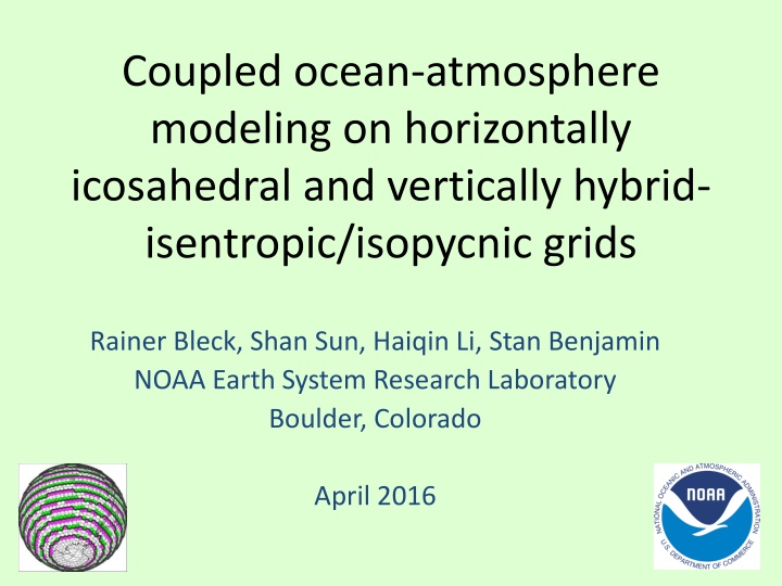
Coupled ocean-atmosphere modeling on horizontally icosahedral and vertically hybrid- isentropic/isopycnic grids Rainer Bleck, Shan Sun, Haiqin Li, Stan Benjamin NOAA Earth System Research Laboratory Boulder, Colorado April 2016
Design goals: (some reached, some pending) Global domain No grid mismatch at ocean-atmo interface Same horizontal resolution as medium-range NWP models (=> eddy-permitting ocean) Envisioned forecast time range: 1 day - 1 month Intrinsic model climate & variability similar to observed Deemed important for reducing biases even in simulations as short as 1 month. Key variability indicators: ENSO, MJO, wintertime stratospheric warming, tropospheric blocking freq. Steadiness of meridional overturning circulations (Hadley, Brewer-Dobson, thermohaline circ.)
The coupled model Atmosphere: FIM (F=flow-following, I=icosahedral) Horizontal grid: icosahedral; resolution choices 240, 120, 60, 30, 15 km (104 - 2.5x10⁶grid cells) Vertical grid: isentropic aloft, reverting to terrain-following near the ground. Adaptive, 64 layers. Ocean: i-HYCOM (icosahedral version of Hybrid Coordinate Ocean Model) Horizontal grid: same as atmosphere Vertical grid: isopycnic at depth, reverting to p near the sea surface. Adaptive, 32 layers. Flux Coupler: a non-issue (matching grid cells!) important: no coastline ambiguities Atmosphere in charge of computing surface fluxes No flux adjustment or post-mortem bias removal
Additional model details -- atmosphere Designed and used at NOAA-ESRL as medium-range NWP model (http://fim.noaa.gov) Hydrostatic. Arakawa-A grid (all variables carried in grid cell center). Finite-volume numerics (2ndorder). Column physics imported from GFS (NOAA-NCEP). Rudimentary river-routing scheme Essential for closing freshwater cycle (=> ocean salinity). Indirect addressing (table lookup) for lateral neighbor interactions. Efficiently parallelized.
Additional model details -- ocean Essentially HYCOM, but rewritten for icosahedral mesh. Vertical coordinate: potential density ( pot) referenced to 1km depth. d pot/dt=0 in adiab.flow (i.e. incompressible w.r.t. pot) Prognostic variables: T, S, u, v, dp (layer thickness). Basic 1-layer ice model, free drift. Simplified barotropic-baroclinic mode splitting 3D equations for u,v,dp solved on barotropic time steps. Bonus: no need to express freshwater fluxes as virtual salt fluxes. Software engineering innovations (parallelization etc.) inherited from FIM. Tightly coupled to atmosphere on baroclinic time steps.
1. Short-range application: Hurricane Chosen example: Hurricane Sandy, October 2012 Initial state (ocean and atmosphere) from NOAA-NCEP Climate Forecast System v.2 Model resolution ~15km. Ocean is eddy-permitting, but no realistic eddies in initial state.
Sample results Hurrican e Sandy 1 triangle=0.5Pa 1 triangle=25cm/s Wind stress (left) and surface currents (right) off the U.S. east coast in 5.5 day forecast starting at 12GMT, 23 Oct 2012. Note: ocean response dominated by inertial waves. No hurricane-induced vortex.
Sample results Surface temperature (left) and salinity (right) in 5.5 day forecast starting at 12GMT, 23 Oct 2012. Note: SST appears to be mainly controlled by cloudiness/precip, not wind stress.
1st layer thickness: 2m Gulf Stream front Zonal vertical section at 370N showing temperature and coordinate layer interfaces. Top section is blowup of bottom section. Note shallowness of srfc. cold layer.
2. Medium-range application: Does intrinsic model variability change over time?
Frequency of blocking episodes (Pelly-Hoskins) in 600 30-day coupled simulations spread over years 1999-2010. Mesh size 30km
3. Long-range application: Does the model support the leading coupled mode in the ocean- atmosphere system?
Grell-Freitas cloud parameterization: mod 2 Grell-Freitas cloud parameterization: mod 3 Top: Nino3 index from final 50-yr period of coupled simulations. Mesh size 120km. Bottom: observed index.
Does the model maintain a reasonably steady Atlantic meridional overturning circulation?
Units: 1 Sverdrup = 106m3/s Time series of oceanic mass flux (Atlantic overturning, Drake Passage, Lombok Strait) in multi-decadal coupled simulation. Mesh size 120km. Note low AMOC (25% of observed strength)
low/high vertical diffusivity Which component of the coupled model is responsible for the low AMOC? Shown here are two ocean-only simulations, forced by observed atmosphere (CORE-II). AMOC is acceptable in this case.
Salinity trends in concentration basins result from precip/evaporation imbalances. Are they tolerable?
Sea surface temperature in concentration basins Year 0 Year 10 Year 20
Sea surface salinity in concentration basins Year 0 Year 10 Year 20 Capping of salinity required here, other basins OK.
Conclusions and Outlook Converting a weather model into a GCM is a challenge, especially when coupling it to an ocean Surface fluxes thrown away in atmo-only applications suddenly become important Column physics codes written for NWP are not necessarily conservative (energy, freshwater cycle) Convective cloud parameterization requires intensive tuning to achieve zero net radiation balance Simulation of ENSO variability moderately successful. Subtle decrease in blocking frequency with forecast duration on monthly time scale. Model maintains weak AMOC on decadal time scales. By using a unique combination of nonstandard 3D grids (icosahedral + isentropic/isopycnic) we strive to contribute to the genetic diversity in coupled multi- model ensemble applications.
