Bayesian Reasoning and Decision Making with Uncertainty
Exploring Bayesian reasoning principles such as Bayesian inference and Naïve Bayes algorithm in the context of uncertainty. The content covers the sources of uncertainty, decision-making strategies, and practical examples like predicting alarm events based on probabilities.

Download Presentation

Please find below an Image/Link to download the presentation.
The content on the website is provided AS IS for your information and personal use only. It may not be sold, licensed, or shared on other websites without obtaining consent from the author.If you encounter any issues during the download, it is possible that the publisher has removed the file from their server.
You are allowed to download the files provided on this website for personal or commercial use, subject to the condition that they are used lawfully. All files are the property of their respective owners.
The content on the website is provided AS IS for your information and personal use only. It may not be sold, licensed, or shared on other websites without obtaining consent from the author.
E N D
Presentation Transcript
Bayesian Reasoning Chapter 13 Thomas Bayes, 1701-1761 1
Todays topics Review probability theory Bayesian inference From the joint distribution Using independence/factoring From sources of evidence Na ve Bayes algorithm for inference and classification tasks 2
Many Sources of Uncertainty Uncertain inputs -- missing and/or noisy data Uncertain knowledge Multiple causes lead to multiple effects Incomplete enumeration of conditions or effects Incomplete knowledge of causality in the domain Probabilistic/stochastic effects Uncertain outputs Abduction and induction are inherently uncertain Default reasoning, even deductive, is uncertain Incomplete deductive inference may be uncertain Probabilistic reasoning only gives probabilistic results 3
Decision making with uncertainty Rational behavior: For each possible action, identify the possible outcomes Compute the probability of each outcome Compute the utility of each outcome Compute the probability-weighted (expected) utility over possible outcomes for each action Select action with the highest expected utility (principle of Maximum Expected Utility) 4
Consider Your house has an alarm system It should go off if a burglar breaks into the house It can go off if there is an earthquake How can we predict what s happened if the alarm goes off?
Probability theory 101 Random variables Domain Atomic event: complete specification of state Prior probability: degree of belief without any other evidence or info Joint probability: matrix of combined probabilities of set of variables Alarm, Burglary, Earthquake Boolean (like these), discrete, continuous Alarm=T Burglary=T Earthquake=F alarm burglary earthquake P(Burglary) = 0.1 P(Alarm) = 0.1 P(earthquake) = 0.000003 P(Alarm, Burglary) = alarm alarm burglary .09 .01 burglary .1 .8 6
alarm alarm Probability theory 101 burglary .09 .01 burglary .1 .8 Conditional probability: prob. of effect given causes Computing conditional probs: P(a | b) = P(a b) / P(b) P(b): normalizing constant Product rule: P(a b) = P(a | b) * P(b) P(burglary | alarm) = .47 P(alarm | burglary) = .9 P(burglary | alarm) = P(burglary alarm) / P(alarm) = .09/.19 = .47 P(burglary alarm) = P(burglary | alarm) * P(alarm) = .47 * .19 = .09 P(alarm) = P(alarm burglary) + P(alarm burglary) = .09+.1 = .19 Marginalizing: P(B) = aP(B, a) P(B) = aP(B | a) P(a) (conditioning) 7
Example: Inference from the joint alarm alarm earthquake earthquake earthquake earthquake burglary .01 .08 .001 .009 burglary .01 .09 .01 .79 P(burglary | alarm) = P(burglary, alarm) = [P(burglary, alarm, earthquake) + P(burglary, alarm, earthquake) = [ (.01, .01) + (.08, .09) ] = [ (.09, .1) ] Since P(burglary | alarm) + P( burglary | alarm) = 1, = 1/(.09+.1) = 5.26 (i.e., P(alarm) = 1/ = .19 quizlet: how can you verify this?) P(burglary | alarm) = .09 * 5.26 = .474 P( burglary | alarm) = .1 * 5.26 = .526 8
Consider A student has to take an exam She might be smart She might have studied She may be prepared for the exam How are these related?
Exercise: Inference from the joint smart smart p(smart study prep) study study study study prepared .432 .16 .084 .008 prepared .048 .16 .036 .072 Queries: What is the prior probability of smart? What is the prior probability of study? What is the conditional probability of prepared, given study and smart? 10
Exercise: Inference from the joint smart smart p(smart study prep) study study study study prepared .432 .16 .084 .008 prepared .048 .16 .036 .072 Queries: What is the prior probability of smart? What is the prior probability of study? What is the conditional probability of prepared, given study and smart? p(smart) = .432 + .16 + .048 + .16 = 0.8 11
Exercise: Inference from the joint smart smart p(smart study prep) study study study study prepared .432 .16 .084 .008 prepared .048 .16 .036 .072 Queries: What is the prior probability of smart? What is the prior probability of study? What is the conditional probability of prepared, given study and smart? 12
Exercise: Inference from the joint smart smart p(smart study prep) study study study study prepared .432 .16 .084 .008 prepared .048 .16 .036 .072 Queries: What is the prior probability of smart? What is the prior probability of study? What is the conditional probability of prepared, given study and smart? p(study) = .432 + .048 + .084 + .036 = 0.6 13
Exercise: Inference from the joint smart smart p(smart study prep) study study study study prepared .432 .16 .084 .008 prepared .048 .16 .036 .072 Queries: What is the prior probability of smart? What is the prior probability of study? What is the conditional probability of prepared, given study and smart? 14
Exercise: Inference from the joint smart smart p(smart study prep) study study study study prepared .432 .16 .084 .008 prepared .048 .16 .036 .072 Queries: What is the prior probability of smart? What is the prior probability of study? What is the conditional probability of prepared, given study and smart? p(prepared|smart,study)= p(prepared,smart,study)/p(smart, study) = .432 / (.432 + .048) = 0.9 15
Independence When variables don t affect each others probabil- ities, we call them independent, and can easily compute their joint and conditional probability: Independent(A, B) P(A B) = P(A) * P(B) or P(A|B) = P(A) {moonPhase, lightLevel} might be independent of {burglary, alarm, earthquake} Maybe not: burglars may be more active during a new moon because darkness hides their activity But if we know light level, moon phase doesn t affect whether we are burglarized If burglarized, light level doesn t affect if alarm goes off Need a more complex notion of independence and methods for reasoning about the relationships 16
Exercise: Independence smart smart p(smart study prep) study study study study prepared .432 .16 .084 .008 prepared .048 .16 .036 .072 Queries: Q1: Is smart independent of study? Q2: Is prepared independent of study? How can we tell? 17
Exercise: Independence smart smart p(smart study prep) study study study study prepared .432 .16 .084 .008 prepared .048 .16 .036 .072 Q1: Is smart independent of study? You might have some intuitive beliefs based on your experience You can also check the data Which way to answer this is better? 18
Exercise: Independence smart smart p(smart study prep) study study study study prepared .432 .16 .084 .008 prepared .048 .16 .036 .072 Q1: Is smart independent of study? Q1 true iff p(smart|study) == p(smart) p(smart|study) = p(smart,study)/p(study) = (.432 + .048) / .6 = 0.8 0.8 == 0.8, so smart is independent of study 19
Exercise: Independence smart smart p(smart study prep) study study study study prepared .432 .16 .084 .008 prepared .048 .16 .036 .072 Q2: Is prepared independent of study? What is prepared? Q2 true iff 20
Exercise: Independence smart smart p(smart study prep) study study study study prepared .432 .16 .084 .008 prepared .048 .16 .036 .072 Q2: Is prepared independent of study? Q2 true iff p(prepared|study) == p(prepared) p(prepared|study) = p(prepared,study)/p(study) = (.432 + .084) / .6 = .86 0.86 0.8, so prepared not independent of study
Conditional independence Absolute independence: A and B are independent if P(A B) = P(A) * P(B); equivalently, P(A) = P(A | B) and P(B) = P(B | A) A and B are conditionally independent given C if P(A B | C) = P(A | C) * P(B | C) This lets us decompose the joint distribution: P(A B C) = P(A | C) * P(B | C) * P(C) Moon-Phase and Burglary are conditionally independent given Light-Level Conditional independence is weaker than absolute independence, but useful in decomposing full joint probability distribution
Conditional independence Intuitive understanding: conditional independence often arises due to causal relations Moon phase causally effects light level at night Other things do too, e.g., street lights For our burglary scenario, moon phase doesn t effect anything else Knowing light level means we can ignore moon phase in predicting whether or not alarm suggests we had a burglary
Bayes rule Derived from the product rule: C is a cause, E is an effect P(C, E) = P(C|E) * P(E) # from definition of conditional probability P(E, C) = P(E|C) * P(C) # from definition of conditional probability P(C, E) = P(E, C) # since order is not important So P(C|E) = P(E|C) * P(C) / P(E) 24
Bayes rule Derived from the product rule: P(C|E) = P(E|C) * P(C) / P(E) Useful for diagnosis: If E are (observed) effects and C are (hidden) causes, Often have model for how causes lead to effects P(E|C) May also have prior beliefs (based on experience) about frequency of causes (P(C)) Which allows us to reason abductively from effects to causes (P(C|E)) 25
Ex: meningitis and stiff neck Meningitis (M) can cause stiff neck (S), though there are other causes too Use S as a diagnostic symptom and estimate p(M|S) Studies can estimate p(M), p(S) & p(S|M), e.g. p(M)=0.7, p(S)=0.01, p(M)=0.00002 Harder to directly gather data on p(M|S) Applying Bayes Rule: p(M|S) = p(S|M) * p(M) / p(S) = 0.0014 26
Bayesian inference In the setting of diagnostic/evidential reasoning i H ) | ( i E P ) hypotheses ( P H i jH evidence/m anifestati ons E E E 1 j m ( ( ( ) | | P P P H E H i jH iE Know prior probability of hypothesis conditional probability Want to compute the posterior probability Bayes s theorem: P(Hi|Ej)= P(Hi)*P(Ej|Hi)/P(Ej) ) ) i j
Simple Bayesian diagnostic reasoning AKA Naive Bayes classifier Knowledge base: Evidence / manifestations: E1, Em Hypotheses / disorders: H1, Hn Note: Ej and Hi are binary; hypotheses are mutually exclusive (non-overlapping) and exhaustive (cover all possible cases) Conditional probabilities: P(Ej | Hi), i = 1, n; j = 1, m Cases (evidence for a particular instance): E1, , El Goal: Find the hypothesis Hi with highest posterior Maxi P(Hi | E1, , El) 28
Simple Bayesian diagnostic reasoning Bayes rule says that P(Hi | E1 Em) = P(E1 Em | Hi) P(Hi) / P(E1 Em) Assume each evidence Ei is conditionally indepen- dent of the others, given a hypothesis Hi, then: P(E1 Em | Hi) = mj=1 P(Ej | Hi) If we only care about relative probabilities for the Hi, then we have: P(Hi | E1 Em) = P(Hi) mj=1 P(Ej | Hi) 29
Limitations Can t easily handle multi-fault situations or cases where intermediate (hidden) causes exist: Disease D causes syndrome S, which causes correlated manifestations M1 and M2 Consider composite hypothesis H1 H2, where H1 & H2independent. What s relative posterior? P(H1 H2 | E1, , El) = P(E1, , El | H1 H2) P(H1 H2) = P(E1, , El | H1 H2) P(H1) P(H2) = lj=1 P(Ej | H1 H2) P(H1) P(H2) How do we compute P(Ej | H1 H2) ? 30
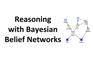
Limitations Assume H1 and H2 are independent, given E1, , El? P(H1 H2 | E1, , El) = P(H1 | E1, , El) P(H2 | E1, , El) Unreasonable assumption Earthquake & Burglar independent, but not given Alarm: P(burglar | alarm, earthquake) << P(burglar | alarm) Doesn t allow causal chaining: A: 2017 weather; B: 2017 corn production; C: 2018 corn price A influences C indirectly: A B C P(C | B, A) = P(C | B) Need richer representation for interacting hypoth- eses, conditional independence & causal chaining Next: Bayesian Belief networks! 31
Summary Probability is a rigorous formalism for uncertain knowledge Joint probability distribution specifies probability of every atomic event Can answer queries by summing over atomic events But we must find a way to reduce joint size for non- trivial domains Bayes rule lets us compute from known conditional probabilities, usually in causal direction Independence & conditional independence provide tools Next: Bayesian belief networks 32