Bayesian Optimization at LCLS Using Gaussian Processes
Bayesian optimization is being used at LCLS to tune the Free Electron Laser (FEL) pulse energy efficiently. The current approach involves a tradeoff between human optimization and numerical optimization methods, with Gaussian processes providing a probabilistic model for tuning strategies. Prior mean Gaussian process parameters and techniques for tuning from noise using historical data are explored, alongside sampling statistics for measuring FEL pulse energy.

Download Presentation

Please find below an Image/Link to download the presentation.
The content on the website is provided AS IS for your information and personal use only. It may not be sold, licensed, or shared on other websites without obtaining consent from the author.If you encounter any issues during the download, it is possible that the publisher has removed the file from their server.
You are allowed to download the files provided on this website for personal or commercial use, subject to the condition that they are used lawfully. All files are the property of their respective owners.
The content on the website is provided AS IS for your information and personal use only. It may not be sold, licensed, or shared on other websites without obtaining consent from the author.
E N D
Presentation Transcript
Bayesian Optimization at LCLS using Gaussian Processes Optimization of FEL pulse energy Joseph Duris, Mitch McIntire, Daniel Ratner ICFA mini-workshop on machine learning for accelerators Feb 28, 2018
Bayesian Optimization Current approach to tuning: One objective: FEL pulse energy Mostly operator controlled Optimization is slow and costly Action Time (mins) Controller Search space Ocelot optimizer Collaboration with DESY Local simplex optimizer Small batches of devices Config change 10 Operators small Tune to find FEL 5-10 Operators large Tune quads 15 Simplex 24 Undulator tuning 5-10 Operators 30 Pointing / focusing 5 Operators small Example opportunities for time savings 2
Bayesian Optimization Tuning strategy tradeoffs Human optimization - mental models - experience - (relatively) slow execution Numerical optimization - fast execution - blind, local search limited search space Bayesian optimization Gaussian process provides probabilistic model GP probabilities + Bayes rule enables use of prior knowledge Acquisition function uses resulting probabilities to guide search 3
Prior mean GP needs 2 key parameters: kernel and prior mean. Ample training data available with wide range of tuned configs from historical tuning. Prior mean biases and constrains search Widths of scans => GPkernel parameters Trends in peaks of scans=> GP prior mean 4
Using the prior mean to tune up from noise We used a Bayes prior from summer 2017 data to tune up a brand new config from noise. Simplex could not do this as it needs signal to tune on. Beam power L3 energy Change 14 -> 6.5 GeV GDET noise? GDET ~ 50 uJ GP run on LI26 quads GP run on LTU quads 5
Sampling statistics Measure FEL pulse energy with gas detector Collection efficiency is small => shot noise dominates Variance proportional to amplitude => std dev is wider Moral of story: sample near the high end of the distribution 6
Tuning 12 quads starting with 30% of peak FEL Simplex GP, expected improvement, Jan 2018 prior 80th percentile of 120 shots Mean of 120 shots 7
Tuning 12 quads starting with 10% of peak FEL GP, expected improvement, Jan 2018 prior GP, UCB Jan 2018 prior Simplex 80th percentile of 120 shots Mean of 120 shots 8
Accommodating correlations between devices n devices FEL vs quads with RBF kernel n x n kernel matrix Current implementation uses diagonal kernel matrix => ignores correlations between quads One approach: vary kernel matrix elements to maximize marginal likelihood for a set of prior scans Another approach: map x to linearly independent basis y with diagonal kernel matrix 9
Tuning the kernel parameters Gaussian process kernel fitting is done via maximum likelihood estimation. The maximum likelihood estimator (MLE) is useful since it is asymptotically normal, is unbiased, is consistent, GP gives likelihood of observations y given samples X and kernel parameters Each scan is potentially a unique set of points, yet the characteristic shape of the function remains similar. Determine kernel parameters (and uncertainties) which maximize net likelihood for a group of scans Work in progress 10
Testing acquisition strategies offline Monte-Carlo platform to investigate optimization strategies offline (i.e. acquisition function parameters) 50 Gaussian processes on simulated data (1mJ peak) with 8 quads GP with prior mean optimizing 10 quads Simplex optimizing 10 quads Optimize trends in offline MC runs to determine best acquisition function parameters. 11
GP progress Prior mean: fits to aggregate historical data Kernel parameters Simultaneous GP likelihood maximization for group of scans determines kernel parameters Monte Carlo Sims => tune acquisition function parameters Expand use-cases Tune quads to minimize beam losses Tuning quads, undulator taper to maximize FEL pulse energy Self-seeding optics vs. FEL peak brightness Control x-ray optics to maximize experimental signal 12
Improving GP flexibility Arbitrary devices may not be related linearly. Example: FEL ~ f(quads / energy) A neural network kernel is a non-linear mapping which can help capture these more complicated relations between input parameters. GP equivalent to a single layer with infinite nodes Rich adaptive basis functions from DNN map on inputs structures data Deep Kernel Learning. Wilson, Hu, Salakhutdinov, Xing. arXiv:1511.02222 The LDRD is now supporting a Stanford CS masters student (Mitch McIntire) working on implementing this kernel to improve the generality of GP to arbitrary inputs. 14
Model selection Gaussian process kernel fitting is done via maximum likelihood estimation. The maximum likelihood estimator (MLE) is useful since it is efficient, Is asymptotically normal, is unbiased, is consistent, Furthermore since the likelihood is normalized, it automatically regularizes. This gives us a statistically sound way to choose our model and give meaningful parameter confidence interval estimates. Example: 15
Gaussian Process components Bayesian optimization with instance based learning Gaussian process provides probabilistic model based on kernel learning GP probabilities + Bayes rule enables use of prior knowledge probability Acquisition function uses resulting probabilities to guide search Acquisition point Acquisition point Acquisition point Acquisition point Acquisition point Acquisition point Acquisition point Acquisition point Acquisition point Acquisition function Ground truth Posterior 16