Cloud-based Geospatial Query Processing Using MapReduce and Voronoi Diagrams

This research paper presents a cloud-based approach for processing geospatial queries efficiently using MapReduce and Voronoi diagrams. The motivation behind the study, related works in the field, preliminary concepts of MapReduce, Voronoi diagram creation, query types, performance evaluation, and future work are discussed. The study focuses on leveraging the scalable nature of cloud platforms to handle large volumes of geo-tagged data and parallelize geospatial queries for improved efficiency.

Download Presentation

Please find below an Image/Link to download the presentation.
The content on the website is provided AS IS for your information and personal use only. It may not be sold, licensed, or shared on other websites without obtaining consent from the author. Download presentation by click this link. If you encounter any issues during the download, it is possible that the publisher has removed the file from their server.
E N D
Presentation Transcript
Afsin Akdogan, Ugur Demiryurek, Farnoush Banaei-Kashani and Cyrus Shahabi University of Southern California 12/02/2011 IBM Student Workshop for Frontiers of Cloud Computing
Outline Motivation Related Work Preliminaries Voronoi Diagram (Index) Creation Query Types Performance Evaluation Conclusion and Future Work
Motivation Size of geo-tagged data rapidly grows. Advances in location-based services. Ex: gps devices, facebook check-in, twitter, etc. Applications of geospatial queries: GIS, Decision support systems, Bioinformatics, etc.
Motivation Geospatial queries on Cloud Big data Geospatial queries are intrinsically parallelizable
Motivation Split 1 Split 2 Problem: Find nearest neighbor of every point. p1 p2 Na ve Solution: Calculate a distance value from p1 to every other point in the map step and find the minimum in the reduce step. Large intermediate result.
Related Work Centralized Systems M. Sharifzadeh and C. Shahabi. VoRTree: Rtrees with Voronoi Diagrams for Efficient Processing of Spatial Nearest Neighbor Queries. VLDB, 2010. Parallel and Distributed Systems Parallel Databases J.M. Patel. Building a Scalable Geospatial Database System. SIGMOD, 1997. Distributed Systems C. Mouza, W. Litwin and P. Rigaux. SD-Rtree: A Scalable Distributed Rtree. ICDE, 2007. Cloud Platforms A. Cary, Z. Sun, V. Hristidis and N. Rishe. Experiences on Processing Spatial Data with MapReduce. SSDBM, 2009.
Our Approach MapReduce-based. Points are in 2D Euclidean space. Data are indexed with Voronoi diagrams. Both Index creation and query processing are done with MapReduce. 3 types of queries: Reverse Nearest Neighbor. Maximizing Reverse Nearest Neighbor (First implementation on a non-centralized system). K-Nearest Neighbor Query.
Outline Motivation Related Work Preliminaries Voronoi Diagram (Index) Creation Query Types Performance Evaluation Conclusion and Future Work
Preliminaries: MapReduce Map(k1,v1) -> list(k2,v2) Reduce(k2, list (v2)) -> list(v3)
Preliminaries: Voronoi Diagrams Given a set of spatial objects, a Voronoi diagram uniquely partitions the space into disjoint regions (cells). The region including object p includes all locations which are closer to p than to any other object p . Ordinary Voronoi diagram Dataset: Points Distance D(.,.): Euclidean Voronoi Cell of p
Preliminaries: Voronoi Diagrams A point cannot have more than 6 Voronoi neighbors on average. Limited search space! Ordinary Voronoi diagram Dataset: Points Distance D(.,.): Euclidean Voronoi Cell of p
Preliminaries: Voronoi Diagrams Nearest Neighbor of p is among its Voronoi neighbors (VN). VN(p) = {p1, p2, p3, p4, p5, p6} p6 p1 p5 p2 p4 p3
Preliminaries: Voronoi Diagrams Nearest Neighbor of p is among its Voronoi neighbors (VN). VN(p) = {p1, p2, p3, p4, p5, p6} p6 p1 p5 p2 p4 p3
Preliminaries: Voronoi Diagrams Nearest Neighbor of p is among its Voronoi neighbors (VN). VN(p) = {p1, p2, p3, p4, p5, p6} p5 is p s nearest neighbor. p6 p1 p5 p2 p4 p3
Outline Motivation Related Work Preliminaries Voronoi Diagram (Index) Creation Query Types Performance Evaluation Conclusion and Future Work
Voronoi Generation: Map phase Generate Partial Voronoi Diagrams (PVD) Split 1 Split 2 right left p7 p1 p3 p5 p8 p4 p2 p6 right left emit emit <key, value>: <1, PVD(Split 1)> <key, value>: <1, PVD(Split 2)>
Voronoi Generation: Reduce phase Remove superfluous edges and generate new edges. Split 1 Split 2 right left p7 p1 p3 p5 p8 p4 p2 p6 right left emit <key, value>: <point, Voronoi Neighbors> <p1, {p2, p3}> <p2, {p1, p3, p4}> <p3, {p1, p2, p4, p5}> ..
Query Type 1: Reverse Nearest Neighbor Given a query point q, Reverse Nearest Neighbor Query finds all points that have q as their nearest neighbors. NN(p1) = p2 NN(p2) = p5 NN(p3) = p5 NN(p4) = p5 NN(p5) = p3 Reverse Nearest Neighbors of p5: {p2, p3, p4} p2 p3 p5 p1 p4
Query Type 1: Reverse Nearest Neighbor How does Voronoi Diagram help? Find Nearest Neighbor of a point p Without Voronoi Diagrams: p2 Calculate a distance value from p to every other point in the map step and find the minimum in the reduce step. p3 p5 p1 p4 Large intermediate result.
Query Type 1: Reverse Nearest Neighbor Map Phase: Input: <point, Voronoi Neighbors> Each point p finds its Nearest Neighbor Emit: <NN(pn), pn> Ex: <p5, p2> <p5, p3> <p5, p4> Reduce Phase: p2 p3 p5 p1 p4 <point, Reverse Nearest Neighbors> Ex: <p5, {p2, p3, p4}>
Query Type 2: MaxRNN Motivation behind parallelization: It requires to process a large dataset in its entirety that may result in an unreasonable response time. In a recent study, it has been showed that the computation of MaxRNN takes several hours for large datasets.
Query Type 2: MaxRNN Locates the optimal region A such that when a new point p is inserted in A, the number of Reverse Nearest Neighbors for p is maximized. Known as the optimal location problem. D A C Region B is maximizing the number of Reverse Nearest Neighbors B p1 p2
Query Type 2: MaxRNN The optimal region can be represented with intersection points that have been overlapped by the highest number of circles. p1 p2 p3 Intersection point
Query Type 2: MaxRNN 2 step Map/Reduce Solution 1. step finds the NN of every point and computes the radiuses of the circles. 2. step finds the overlapping circles first. Then, it finds the intersection points that represent the optimal region. Runs several times.
Outline Motivation Related Work Preliminaries Voronoi Diagram (Index) Creation Query Types Performance Evaluation Conclusion and Future Work
Performance Evaluation Real-World Navteq datasets: BSN: all businesses in the entire U.S., containing approximately 1,300,000 data points. RES: all restaurants in the entire U.S., containing approximately 450,000 data points. Hadoop on Amazon EC2 Evaluated our approach based on Index Generation Query Response times Replication factor = 1
Performance Evaluation Voronoi Index Competitor approach: MapReduce based Rtree RTree generation is faster than Voronoi. Voronoi is better in Query Response times (Ex: Reverse Nearest Neighbor) Nearest Neighbor of every point
Performance Evaluation MaxRNN First implementation on a non-centralized system. Evaluated the performance for 2 different datasets. 12 Execution time (min) BSN RES 10 8 6 4 2 0 2 4 8 16 32 Node number
Conclusion and Future Work Conclusion Geospatial Queries are parallelizable. Indexing (Voronoi Diagram) significantly improves the performance. Ongoing Work Scalable Distributed Index Structure for spatial data.