Understanding Population Growth Models and Stochastic Effects
Explore the simplest model of population growth and the assumptions it relies on. Delve into the challenges of real-world scenarios, such as stochastic effects caused by demographic and environmental variations in birth and death rates. Learn how these factors impact predictions and models.
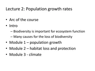
- Population growth
- Stochastic effects
- Demographic stochasticity
- Environmental stochasticity
- Assumptions

Download Presentation

Please find below an Image/Link to download the presentation.
The content on the website is provided AS IS for your information and personal use only. It may not be sold, licensed, or shared on other websites without obtaining consent from the author. Download presentation by click this link. If you encounter any issues during the download, it is possible that the publisher has removed the file from their server.
E N D
Presentation Transcript
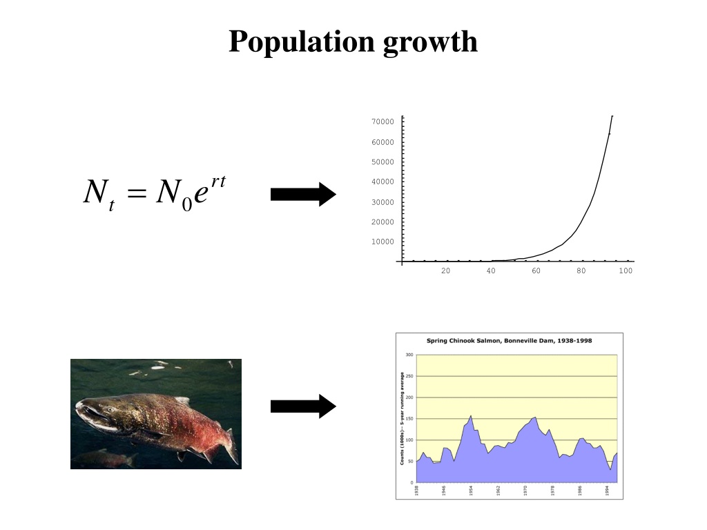
Population growth 70000 60000 50000 = rt N N e 40000 0 t 30000 20000 10000 20 40 60 80 100
The simplest model of population growth dN = = ( ) b d N rN dt dN dt What are the assumptions of this model?
We already saw that the solution is: = rt N N e 0 t 70000 60000 50000 N 40000 dN 30000 dt 20000 10000 20 40 60 80 100 t r determines how rapidly the population will increase
A test of the exponential model: Pheasants on Protection Island Abundant food resources Exponential prediction No bird predators No migration 8 pheasants introduced in 1937 Observed By 1942, the exponential model overestimated the # of birds by 4035
Where did the model go wrong? Assumptions of our simple model: 1. No immigration or emigration 2. Constant r - - No random/stochastic variation Constant supply of resources 3. No genetic structure (all individuals have the same r) 4. No age or size structure
Stochastic effects In real populations, r is likely to vary from year to year as a result of random variation in the per capita birth and death rates, b and d. This random variation can be generated in two ways: 1. Demographic stochasticity Random variation in birth and death rates due to sampling error in finite populations 2. Environmental stochasticity Random variation in birth and death rates due to random variation in environmental conditions
I. Demographic stochasticity Imagine a population with an expected per capita birth rate of b = 2 and an expected per capita death rate of d = 0. In an INFINITE population, the average value of b is 2, even though some individuals have less than 2 offspring per unit time and some have more.
I. Demographic stochasticity But in a FINITE population, say of size 2, this is not necessarily the case! Here, b = 2.5 (different from its expected value of 2) solely because of RANDOM chance!
I. Demographic stochasticity Imagine a case where females produce, on average, 1 male and 1 female offspring. In an INFINITE population the average value of b = 1, even though some individuals have less than 1 female offspring per unit time and some have more N=0
I. Demographic stochasticity But in a FINITE population, say of size 2, this is not necessarily the case! If the finite population were just these two Here, b = .5 (different from its expected value of 1) solely because of RANDOM chance!
II. Environmental stochasticity r is a function of current environmental conditions Does not require FINITE populations Anderson, J.J. 1995. Decline and Recovery of Snake River Salmon. Information based on the CRiSP research project. Testimony before the U.S. House of Representatitives Subcommittee on Power and Water, June 3. Source:
How important is stochasticity? An example from the wolves of Isle Royal (Vucetich and Peterson, 2004) Map of Isle Royale No immigration or emigration Wolves eat only moose Moose are only eaten by wolves
How important is stochasticity? An example from the wolves of Isle Royal Wolf population sizes fluctuate rapidly Moose population size also fluctuates What does this tell us about the growth rate, r, of the wolf population?
How important is stochasticity? An example from the wolves of Isle Royal The growth rate of the wolf population, r, is better characterized by a probability distribution with mean, , and variance, . r r V Frequency Growth rate, r What causes this variation in growth rate?
How important is stochasticity? An example from the wolves of Isle Royal The researchers wished to test four hypothesized causes of growth rate variation: 1. Snowfall (environmental stochasticity) 2. Population size of old moose (environmental stochasticity?) 3. Population size of wolves 4. Demographic stochasticity To this end, they collected data on each of these factors from 1971-2001 So what did they find?
How important is stochasticity? An example from the wolves of Isle Royal Cause Percent variation in growth rate explained 42% Old moose Demographic stochasticity Wolves Snowfall Unexplained 30% 8% 3% 17% (Vucetich and Peterson, 2004) In this system, approximately 30% of the variation is due to demographic stochasticity Another 45% is due to what can perhaps be considered environmental stochasticity. *** At least for this wolf population, stochasticity is hugely important***
Practice Problem: You have observed the following pattern Lake 1 Lake 2
In light of this phylogenetic data, how to you hypothesize speciation occurred? Lake X Lake 1 Lake 2 Lake 1 Lake 2
A scenario consistent with the data Lake 1 Lake 2
A scenario consistent with the data Lake 1 Lake 2
A scenario consistent with the data Lake 1 Lake 2
Predicting population growth with stochasticity Stochasticity is important in real populations; how can we integrate this into population predictions? Frequency Growth rate, r = rt N N e In other words, how do we integrate this distribution into: 0 t
Lets look at a single population Imagine a population with an initial size of 10 individuals and an average growth rate of r = .01 In the absence of stochasticity, our population would do this 50 40 30 N 20 10 20 40 60 80 100 t The growth of this population is assured, there is no chance of extinction
But with stochasticity we could get this Vr = 0 Vr = .0025 0.2 0.2 0.1 0.1 r 20 40 60 80 100 20 40 60 80 100 0.1 0.1 0.2 0.2 50 50 40 40 30 30 N 20 20 10 10 20 40 60 80 100 20 40 60 80 100 t t
Or this Vr = 0 Vr = .0025 0.2 0.2 0.1 0.1 r 20 40 60 80 100 20 40 60 80 100 0.1 0.1 0.2 0.2 50 50 40 40 30 30 N 20 20 10 10 20 40 60 80 100 20 40 60 80 100 t t
Or even this Vr = 0 Vr = .0025 0.2 0.2 0.1 0.1 r 20 40 60 80 100 20 40 60 80 100 0.1 0.1 0.2 0.2 50 50 40 40 30 30 N 20 20 10 10 20 40 60 80 100 20 40 60 80 100 t t
Integrating stochasticity Generation 1: Draw r at random calculate the new population size Generation 2: Draw r atrandom calculate the new population size . . . and so on and so forth The result is that we can no longer precisely predict the future size of the population. Instead, we can predict: 1) the expected population size, and 2) the variance in population size. = t r N N e 0 t = ) 1 V t 2 0 2 t r ( V N e e r N t Lets illustrate this with some examples
Comparing two cases = = 05 . 0 r r V Case 1: No stochasticity ( ) 500 1 Frequency 0.8 400 0.6 N 300 0.4 0.2 200 0 100 0 0.1 0.01 0.02 0.03 0.04 0.05 0.06 r 0.07 0.08 0.09 20 40 t 60 80 = = 05 . 0001 . r r V Case 2: Stochasticity ( ) 500 0.3 400 Frequency 0.25 95% of values lie in the shaded area 0.2 300 N 0.15 0.1 200 0.05 100 0 0 0.1 0.01 0.02 0.03 0.04 0.05 0.06 r 0.07 0.08 0.09 20 40 t 60 80
What if the variance in r is increased? = = 05 . 0 r r V Case 1: No stochasticity ( ) 500 1 Frequency 400 0.8 0.6 N 300 0.4 0.2 200 0 100 0 r 0.1 -0.1 0.02 0.04 0.06 0.08 -0.08 -0.06 -0.04 -0.02 20 40 t 60 80 = = 05 . 005 . r r V Case 2: Stochasticity ( ) 500 400 0.3 95% of values lie in the shaded area 0.25 Frequency 300 0.2 N 0.15 200 0.1 0.05 100 0 0 r 0.1 -0.1 0.02 0.04 0.06 0.08 -0.08 -0.06 -0.04 -0.02 20 40 60 80 t
How can we predict the fate of a real population? = t r N N e 0 t = ) 1 V t 2 0 2 t r ( V N e e r N t What kind of data do we need? How could we get this data? How do we plug the data into the equations? How do we make biological predictions from the equations?
A hypothetical data set Photo: Wolverine on a rock Replicate 1 2 3 4 5 6 7 8 9 10 r 0.10 0.15 0.05 0.00 -0.05 -0.02 0.05 -0.08 0.02 -0.05 Wolverine (Gulo gulo) The question: How likely it is that a small (N0 = 46) population of wolverines will persist for 100 years without intervention? The data: r values across ten replicate studies
r Calculation and Vr Replicate 1 2 3 4 5 6 7 8 9 10 r = ? r 0.10 0.15 0.05 0.00 -0.05 -0.02 0.05 -0.08 0.02 -0.05 Vr = ?
Using estimates of and Vr in the equations r = = t r ? N N e 0 t = ) 1 = V t 2 0 2 t r ( ? V N e e r N t
Translating the results back into biology = N 100 = V 100 , N OK, so what do these numbers mean? Remember that, for a normal distribution, 95% of values lie within 1.96 standard deviations of the mean Frequency This allows us to put crude bounds on our estimate for future population size What do we conclude about our wolverines? N100 95% of values lie between these arrow heads
Practice Problem Photo: Wolverine on a rock Replicate 1 2 3 4 5 6 7 8 9 10 r 0.05 0.17 0.01 0.00 -0.07 -0.04 0.01 -0.08 0.02 -0.07 Wolverine (Gulo gulo) The question: How likely it is that a small (N0 = 36) population of wolverines will persist for 80 years without intervention? The data: r values across ten replicate studies