Understanding Random Variables and Probability Distributions
Random variables play a crucial role in statistics, representing outcomes of chance events. This content delves into discrete and continuous random variables, probability distributions, notation, and examples. It highlights how these concepts are used to analyze data and make predictions, emphasizing population distributions and key parameters like mean and variance.

Download Presentation

Please find below an Image/Link to download the presentation.
The content on the website is provided AS IS for your information and personal use only. It may not be sold, licensed, or shared on other websites without obtaining consent from the author. Download presentation by click this link. If you encounter any issues during the download, it is possible that the publisher has removed the file from their server.
E N D
Presentation Transcript
Chapters 1. Introduction 2. Graphs 3. Descriptive statistics 4. Basic probability 5. Discrete distributions 6. Continuous distributions 7. Central limit theorem 8. Estimation 9. Hypothesis testing 10. Two-sample tests 13. Linear regression 14. Multivariate regression Chapter 5 Random Variables and Discrete Probability Distributions
Random Variables (RV) When the value that a variable assumes at the end of an experiment is the result of a chance or random occurrence, that variable is a Random Variable (R.V.) Discrete Random Variable takes on finite or infinite but a countable number of different values E.g. values on the roll of dice: 2, 3, 4, , 12 gaps between values along the number line possible to list all results and the associated probabilities Continuous Random Variable takes on any value in an interval. E.g. time (30.1 minutes? 30.10000001 minutes?) no gaps between values along the number line cannot associate possibility with a single value, only a range of values. Analogy: Integers are Discrete, while Real Numbers are Continuous 9/25/2024 Towson University - J. Jung 7.2
Probability Distributions A probability distribution is a table, formula, or graph that describes the values of a random variable and the probability associated with these values. Since we re describing a random variable (which can be discrete or continuous) we have two types of probability distributions: Discrete Probability Distribution Continuous Probability Distribution 9/25/2024 Towson University - J. Jung 7.3
Probability Notation An upper-case letter will represent the name of the random variable, usually X. Its lower-case counterpart will represent the value of the random variable. The probability that the random variable X will equal x is: P(X = x) or more simply P(x) 9/25/2024 Towson University - J. Jung 7.4
Example 5.1 Probability distributions can be estimated from relative frequencies. Consider the discrete (countable) number of televisions per household from US survey data. E.g. what is the probability there is at least one television but no more than three in any given household? 1,218 101,501=0.012 at least one television but no more than three P(1 X 3) = P(1) + P(2) + P(3) = .319 + .374 + .191 = .884 e.g. P(X=4) = P(4) = 0.076 = 7.6% 9/25/2024 Towson University - J. Jung 7.5
Population/Probability Distribution The discrete probability distribution represents a population Example 5.1 the population of number of TVs per household Since we have populations, we can describe them by computing various parameters. E.g. the population mean and population variance. 9/25/2024 Towson University - J. Jung 7.6
Population Mean (Expected Value) The population mean is the weighted average of all of its values. The weights are the probabilities. This parameter is also called the expected value of X and is represented by E(X). 9/25/2024 Towson University - J. Jung 7.7
Population Variance The population variance is calculated similarly. It is the weighted average of the squared deviations from the mean. As before, there is a short-cut formulation The standard deviation is the same as before: 9/25/2024 Towson University - J. Jung 7.8
Example 5.1 Find the mean, variance, and standard deviation for the population of the number of color televisions per household (from Example 7.1) = 0(.012) + 1(.319) + 2(.374) + 3(.191) + 4(.076) + 5(.028) = 2.084 9/25/2024 Towson University - J. Jung 7.9
Example 5.1 Find the mean, variance, and standard deviation for the population of the number of color televisions per household (from Example 7.1) = (0 2.084)2(.012) + (1 2.084)2(.319)+ +(5 2.084)2(.028) = 1.107 9/25/2024 Towson University - J. Jung 7.10
Laws of Expected Value 1. E(c) = c The expected value of a constant (c) is just the value of the constant. 2. E(X + c) = E(X) + c 3. E(cX) = cE(X) We can pull a constant out of the expected value expression (either as part of a sum with a random variable X or as a coefficient of random variable X). 9/25/2024 Towson University - J. Jung 7.11
Example 5.2 Monthly sales have a mean of $25,000 and a standard deviation of $4,000. Profits are calculated by multiplying sales by 30% and subtracting fixed costs of $6,000. Find the mean monthly profit. sales have a mean of $25,000 E(Sales) = 25,000 profits are calculated by Profit = .30(Sales) 6,000 E(Profit) =E[.30(Sales) 6,000] =E[.30(Sales)] 6,000 =.30E(Sales) 6,000 =.30(25,000) 6,000 = 1,500 Thus, the mean monthly profit is $1,500 [by rule #2] [by rule #3] 9/25/2024 Towson University - J. Jung 7.12
Laws of Variance 1. V(c) = 0 The variance of a constant (c) is zero. 2. V(X + c) = V(X) The variance of a random variable and a constant is just the variance of the random variable (per 1 above). 3. V(cX) = c2V(X) The variance of a random variable and a constant coefficient is the coefficient squared times the variance of the random variable. 9/25/2024 Towson University - J. Jung 7.13
Example 5.2 Monthly sales have a mean of $25,000 and a standard deviation of $4,000. Profits are calculated by multiplying sales by 30% and subtracting fixed costs of $6,000. Find the standard deviation of monthly profits. The variance of profit is = V(Profit) =V[.30(Sales) 6,000] =V[.30(Sales)] =(.30)2V(Sales) =(.30)2(16,000,000) = 1,440,000 Again, standard deviation is the square root of variance, so standard deviation of Sdev(Profit) = (1,440,000)1/2 = $1,200 [by rule #2] [by rule #3] 9/25/2024 Towson University - J. Jung 7.14
Optional 9/25/2024 Towson University - J. Jung 7.15
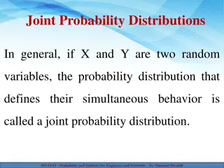
Bivariate Distributions Up to now, we have looked at univariate distributions, i.e. probability distributions in one variable. As you might guess, bivariate distributions are probabilities of combinations of two variables. Bivariate probability distributions are also called joint probability. A joint probability distribution of X and Y is a table or formula that lists the joint probabilities for all pairs of values x and y, and is denoted P(x,y). P(x,y) = P(X=x and Y=y) 9/25/2024 Towson University - J. Jung 7.16
Discrete Bivariate Distribution As you might expect, the requirements for a bivariate distribution are similar to a univariate distribution, with only minor changes to the notation: for all pairs (x,y). 9/25/2024 Towson University - J. Jung 7.17
Example 7.5 Xavier and Yvette are real estate agents; let s use X and Y to denote the number of houses each sells in a month. The following joint probabilities are based on past sales performance: We interpret these joint probabilities as before. E.g the probability that Xavier sells 0 houses and Yvette sells 1 house in the month is P(0, 1) = .21 9/25/2024 Towson University - J. Jung 7.18
Marginal Probabilities As before, we can calculate the marginal probabilities by summing across rows and down columns to determine the probabilities of X and Y individually: E.g the probability that Xavier sells 1 house = P(X=1) =0.50 9/25/2024 Towson University - J. Jung 7.19
Describing the Bivariate Distribution We can describe the mean, variance, and standard deviation of each variable in a bivariate distribution by working with the marginal probabilities same formulae as for univariate distributions 9/25/2024 Towson University - J. Jung 7.20
Covariance The covariance of two discrete variables is defined as: or alternatively using this shortcut method: 9/25/2024 Towson University - J. Jung 7.21
Coefficient of Correlation The coefficient of correlation is calculated in the same way as described earlier 9/25/2024 Towson University - J. Jung 7.22
Example 5.3 Compute the covariance and the coefficient of correlation between the numbers of houses sold by Xavier and Yvette. COV(X,Y) = (0 .7)(0 .5)(.12) + (1 .7)(0 .5)(.42) + + (2 .7)(2 .5)(.01) = .15 = 0.15 [(.64)(.67)] = 0.35 There is a weak, negative relationship between the two variables. 9/25/2024 Towson University - J. Jung 7.23
Laws We can derive laws of expected value and variance for the linear combination of two variables as follows: 1. E(aX + bY) = aE(X) + bE(Y) 2. V(aX + bY) = a2V(X) + b2V(Y) + 2abCOV(X, Y) If X and Y are independent: COV(X, Y) = 0 and thus: V(aX + bY) = a2V(X) + b2V(Y) 9/25/2024 Towson University - J. Jung 7.24
Example 5.3 Suppose the profit for Xavier is $2,000 per house sold, and that for Yvette is $3,000. What is the expected value and variance for the total profit of Xavier and Yvette? Linear combination: TP=2000X+3000Y E(TP)=2000E(X)+3000E(Y)=2000*.7+3000*.5=2900 V(TP)=20002V(X)+30002V(Y)+2*2000*3000*COV(X,Y) =20002*0.41+30002*0.45+2*2000*3000*(-.15) =1640000+4050000-1800000 =3.890,000 9/25/2024 Towson University - J. Jung 7.25

")


")