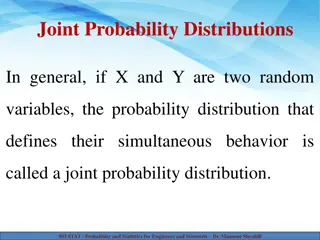
Understanding Random Variables and Probability Distributions

Random variables are variables whose values are unknown and can be discrete or continuous. Probability distributions provide the likelihood of outcomes in a random experiment. Learn how random variables are used in quantifying outcomes and differentiating from algebraic variables. Explore types of random variables and how they play a significant role in statistical analysis.

Download Presentation

Please find below an Image/Link to download the presentation.
The content on the website is provided AS IS for your information and personal use only. It may not be sold, licensed, or shared on other websites without obtaining consent from the author. Download presentation by click this link. If you encounter any issues during the download, it is possible that the publisher has removed the file from their server.
E N D
Presentation Transcript
RANDOM VARIABLE AND PROBABILITY DISTRIBUTIONS CHAPTER 2
RANDOM VARIABLE A random variable is a variable whose value is unknown or a function that assigns values to each of an experiment's outcomes. Random variables are often designated by letters and can be classified as discrete, which are variables that have specific values, or continuous, which are variables that can have any values within a continuous range.
PROBABILITY DISTRIBUTION In Statistics, the probability distribution gives the possibility of each outcome of a random experiment or event. It provides the probabilities of different possible occurrences. Also read, events in probability, here. To recall, the probability is a measure of uncertainty of various phenomena. Like, if you throw a dice, the possible outcomes of it, is defined by the probability. This distribution could be defined with any random experiments, whose outcome is not sure or could not be predicted. Let us discuss now its definition, function, formula and its types here, along with how to create a table of probability based on random variables.
UNDERSTANDING THE RANDOM VARIABLES In probability and statistics, random variables are used to quantify outcomes of a random occurrence, and therefore, can take on many values. Random variables are required to be measurable and are typically real numbers. For example, the letter X may be designated to represent the sum of the resulting numbers after three dice are rolled. In this case, X could be 3 (1 + 1+ 1), 18 (6 + 6 + 6), or somewhere between 3 and 18, since the highest number of a die is 6 and the lowest number is 1.
A random variable is different from an algebraic variable. The variable in an algebraic equation is an unknown value that can be calculated. The equation 10 + x = 13 shows that we can calculate the specific value for x which is 3. On the other hand, a random variable has a set of values, and any of those values could be the resulting outcome as seen in the example of the dice above. Types of Random Variables A random variable can be either discrete or continuous. Discrete random variables take on a countable number of distinct values. Consider an experiment where a coin is tossed three times. If X represents the number of times that the coin comes up heads, then X is a discrete random variable that can only have the values 0, 1, 2, 3 (from no heads in three successive coin tosses to all heads). No other value is possible for X.
Continuous random variables can represent any value within a specified range or interval and can take on an infinite number of possible values. An example of a continuous random variable would be an experiment that involves measuring the amount of rainfall in a city over a year or the average height of a random group of 25 people. Drawing on the latter, if Y represents the random variable for the average height of a random group of 25 people, you will find that the resulting outcome is a continuous figure since height may be 5 ft or 5.01 ft or 5.0001 ft. Clearly, there is an infinite number of possible values for height.
The following is a formal definition. Definition If is a random variable, its distribution function is a function such thatwhere is the probability that is less than or equal to . Example Suppose that a random variable can take only two values (0 and 1), each with probability 1/2. Its distribution function is
Here is a plot of the function.
Properties Every distribution function enjoys the following four properties: Increasing. is increasing, Right-continuous. is right-continuous, Limit at minus infinity. satisfies Limit at plus infinity. satisfies Concise proofs of these properties can be found here and in Williams (1991).
Proper distribution function Any distribution function enjoys the four properties above. Moreover, for any given function enjoying these four properties, it is possible to define a random variable that has the given function as its distribution function (for a proof, see Williams 1991, Sec. 3.11). The practical consequence of this fact is that, when we need to check whether a given function is a proper distribution function, we just need to verify that it satisfies the four properties above.
Example Suppose that the probability mass function of is
Then, we can set up a table that has three rows. In the first row, we write the possible values of , sorted from smallest to largest. In the second row, we write the probabilities of the single values. The third row contains the values of the cdf. The leftmost cell in the third row is equal to the cell immediately above. Then, we go from left to right and the value in each cell is set equal to the sum of: the probability in the cell immediately to the left; the probability in the cell immediately above.
Thus, the distribution function is