Understanding Generalized Linear Models in Psychology and Statistics

Delve into the world of Generalized Linear Models (GLMs) in psychology and statistics with a focus on regression, model assumptions, parameter estimates, and model selection. Explore the application of GLMs in analyzing various types of data, including not normally distributed data, counts, and ordinal data. Discover the significance of GLMs as a statistical tool in research and data analysis.

Download Presentation

Please find below an Image/Link to download the presentation.
The content on the website is provided AS IS for your information and personal use only. It may not be sold, licensed, or shared on other websites without obtaining consent from the author. Download presentation by click this link. If you encounter any issues during the download, it is possible that the publisher has removed the file from their server.
E N D
Presentation Transcript
httpswww.vox.comfuture-perfect21504366science-replication-crisis-peer-httpswww.vox.comfuture-perfect21504366science-replication-crisis-peer- review-statisticsfbclid=IwAR3lIJXfXBVwFWaE5aw4RXHKY GENERALIZED LINEAR MODELS Ph.DProgrammein Psychology, Linguistics and Cognitive Neurosciences Ph.D. School - University of Milano-Bicocca Prof. Franca Crippa
PLAN OF THE LESSON Part I Icebreakers: reviewof the General Linear Models Part II The Generalized linear Model : extension to not normally distributed data. fractions (logistic regression), counts (Poisson regression, log-linear models), ordinal data (threshold models). Overview of specific topics ( overdispersion, (quasi-) maximum likelihood) Part III Overview of software for GLIMs. Spss and in R. Jamoviand Jasp (bothuser-friendly based on some R. R is stillthe Linus blanket, for wideness and updates on modelling, even ifa bit roughand notfluffy. Ph.D. School - University of Milano-Bicocca Prof. Franca Crippa
PART I Icebreaker on the General Linear Model Ph.D. School - University of Milano-Bicocca Prof. Franca Crippa
GENERAL LINEAR MODELS AS MODELS Our idea is that data are generated as specified in our model plus a random error Beware: notation may vary from an author to another, from one professor to another, from one journal to another. DATA = MODEL + ERROR Very general form of the model: ? = ?(??,??, ??)+? Then : focus on the meaning of the symbol; payattention to the requirementsof the journal Linear Models are models ? = ??+????+????+ ????+? Ph.D. School - University of Milano-Bicocca Prof. Franca Crippa
HOW DO WE MODEL DATA? Objective Model structure (e.g. variables, formula, equation) Model assumptions Parameter estimates and interpretation Model fit (e.g. goodness-of-fit tests and statistics) Model selection Ph.D. School - University of Milano-Bicocca Prof. Franca Crippa
PSYCHOLOGISTS STATISTICALWORKHORSE: THE GENERAL LINEAR MODEL Predictors Quantitative predictors - regression quant itativ e quali tativ e Linear regression (simple or multiple) Anova Categorical predictors - ANOVA Ancova both One or more between- subjects predictors Quantitative and categorical predictors - ANCOVA Response: quantative continuous At least one within- subjects predictors Ph.D. School - University of Milano-Bicocca Prof. Franca Crippa
PSYCHOLOGISTS STATISTICALWORKHORSE: THE GENERAL LINEAR MODEL Response: quantativecontinuous One or more dichotomous or continuous between-subjects predictors >=two predictors >=two predictors plus interaction One predictor Multiple regression Interactions Independent samples t-test Simple regression Statistical control (covariates) Moderated mediation Other type of linear model (polynomial) Mediation Ph.D. School - University of Milano-Bicocca Prof. Franca Crippa
THE GENERAL LINEAR MODEL At least one within-subjects predictors An additional random term One or more categorical within-subjects predictors At least one continuous within-subjects predictor Paired-samples t-test Linear Mixed-Effects Models (LMEM) Within-subjects ANOVA 8
GENERAL LINEAR MODEL: AN OUTLOOKON THE ASSUMPTIONS Predictors 1 . on any scale: categorical or quantitative 2. measuredwithouterror(deterministic) random component expressedby the error Response variable: (continuous) quantitative only errors are iid and normally distributed. For all subjects i=1,2,..n. the errors iare: i) ii) identically, normally distributedwith zero meanand equal variance (omoschedasticity) Incorrelated (independent) Objective: the response yi; i = 1, .., n is modelled by a linear (additive) function of predictors/explanatory variables xj ; j = 1, , p plus an error term The model is linear in the parameters Ph.D. School - University of Milano-Bicocca Prof. Franca Crippa
ESTIMATIONWHENASSUMTIONSARE MET The general linear model make the assumptions below. When these assumptions are met, OLS regression coefficients are MVUE (Minimum Variance Unbiased Estimators) and BLUE (Best Linear Unbiased Estimators). 1. Exact X: The IVs are assumed to be known exactly (i.e., without measurement error), deterministic. 2. Independence: Residuals are independently distributed (prob. of obtaining a specific observation does not depend on other observations) 3. Normality: All residual distributions are normally distributed 4. Constant variance: All residual distributions have a constant variance 5. Linearity: All residual distributions (i.e., for each Y') are assumed to have means equal to zero 2. 3. 4. 5.
PARAMETER INTERPRETATION Regression: b0estimate of the intercept ?0 biis estimate of the slope?0, i.e. the increaseof the responsedue to the unitaryincreaseof the i.th preditor Anova General mean Differencebetween the groupmeanand the general mean Model selection: which explanatory variables to include? Principleof parsimony(Occam srazor): allrelevantpredictors are included, no irrelevantoneis. Ph.D. School - University of Milano-Bicocca Prof. Franca Crippa
NOT ALL MISSING DATA ARE THE SAME Missing by design Values are missing by definition of the population of interest Missing completely at random (MCAR) Missing values are randomly distributed Missing at random (MAR) After accounting for one or more other variables, missing values are randomly distributed Non-ignorable (NI) Missing values are functions of the variables themselves
BETTER METHODS OF HANDLING MISSING DATA Full information maximum likelihood (FIML) methods Can handle data that are MAR and NI Implemented as part of particular statistical models Missing data handled during analysis Multiple imputation Can also handle data that are MAR and NI Simulation-based approach Missing data are handled separately from analysis
RESTRICTIONSOF GENERAL LINEAR MODELS Although a very useful framework, there are some situations where general linear models are not appropriate 1. The range of Y is restricted categorical variables, binary, ordered or unordered categories, counts 2. Other violations of assumptions Heteroschedasticity Non-normality Non linearity(in the Ivs and/or in the parameters) Variancedepending on the mean Ph.D. School - University of Milano-Bicocca Prof. Franca Crippa
MESSY DATA Anscombe s quartet Anscombe, Francis J. (1973) Graphs in statistical analysis. American Statistician, 27, 17 21 Ph.D. School - University of Milano-Bicocca Prof. Franca Crippa
A GLANCETO DECISIONAND POWER (NEXT LESSON) Reality: NO EFFECT Reality: EFFECT EXISTS TYPE 2 ERROR ( ) Research concludes: CORRECT FTR FAIL TO REJECT (FTR) NULL; NO EFFECT TYPE 1 ERROR ( ) CORRECT REJECT (1- ) Researcher concludes: REJECT NULL; EFFECT EXISTS 16
PART II GeneralisedLinear Models(GLIMs) Ph.D. School - University of Milano-Bicocca Prof. Franca Crippa
EXTENSION TO GENERALIZED LINEAR MODELS (GLIMOR GLM) GLIMsare a family of models that: Represent an extension of linear regression to a broader family of outcome variables - basic structure of linear regression equations. Allowus to extendthe linear modellingframework to variables that are not Normally distributed. Allow us to look atmodels thatseem different in a unifyingperspective. Two major additions to the linear function framework link function : when the response has a nonlinear relationships with predictors, a transformation of the response is expressed as a linear regression error structures beyond the normally, for instance binomial, poisson. Ph.D. School - University of Milano-Bicocca Prof. Franca Crippa
THREE COMPONENTS OF A GLIM How to approachGLIM: Understanding the common underlyinglinear structure Esploringreason for different estimationtechniques 1. Systematic part: relation between the dependent variableY and the independent variables in the model. 2. Random part: error distribution of the outcome variable 3. Link function: transform of the response, so that the transfom is expressed a the well known linear relation g( ) link function (linear, logit, poisson..) Ph.D. School - University of Milano-Bicocca Prof. Franca Crippa
GLIM FIXED MODELSWITH RESPONSESAND PREDICTORSOF ANYTYPE Predictors measured on any scale. Response General linear model continu ous dichoto mous Logit (accuracy, yes or no) Logistic(ordinal or nominal categorical) categ orical Poissonregression(countvariables, frequencies) count Ph.D. School - University of Milano-Bicocca Prof. Franca Crippa
GLIMASA SOLUTION FOR SOME VIOLATIONSOF GENERAL LINEAR MODELS ASSUMPTIONS (Independence: Inaccurate standard errors, degrees of freedom and significance tests. Use linear mixed effects models see my collegue s lessons) Normality: Inefficient (with large N). Use transformations, generalized linear models Constant variance: Inefficient and inaccurate standard errors. Use transformations, generalized linear models Linearity: Biased parameter estimates. Use transformations, generalized linear models 21
DISTRIBUTION OF ERRORS IN PROBITAND LOGIT MODELS Ph.D. School - University of Milano-Bicocca Prof. Franca Crippa
glm(formula, family=familytype(link=linkfunction), data=) Family binomial gaussian Gamma inverse.gaussian poisson quasibinomial quasipoisson Default Link Function (link = "logit") (link = "identity") (link = "inverse") (link = "1/mu^2") (link = "log") (link = "logit") (link = "log") Ph.D. School - University of Milano-Bicocca Prof. Franca Crippa
LINK FUNCTIONAND ERROR DISTRIBUTIONS model Error distribution Link function Regression Normal g=E(Y|X) ? Binary logisticregression Binomial g=?? 1 ? ? Ordinallogisticregression Binomial g=?? 1 ? ? Multinomiallogisticregression Multinomial g=?? 1 ? Poissonregression Poisson g=ln[E(Y|X)] Beta regression Beta g=ln[E(Y|X)] Gamma regression Gamma g=ln[E(Y|X)] Negative binomial regression Negative binomial g=ln[E(Y|X)] Ph.D. School - University of Milano-Bicocca Prof. Franca Crippa
FIRST CASE: MODELLING THE PROBABILITY FOR A DICHOTOMOUS VARIABLE Family 1. binomial Default Link Function (link = "logit") In a binomialvariable(the random component is the error, whichisbinomial) our interestis on the probabilityof success . In factwehaveto outcomes, success and insuccess(1 and 0). Whenwe knowthe probabilityof success p, thenwederive the probabilityof success as 1-p. Our reponsewould be the probability, range0-1. Then wecannotuse the General Linear Model. How do wesolve the problem? - Wetransformthe response. Insteadof the probability, we considerthe logit g=?? 1 ?. The symbol g standsfor our transformed response. This transformed responsenowis continuous. ? Ph.D. School - University of Milano-Bicocca Prof. Franca Crippa
SECOND CASE: MODELLING THE PROBABILITY FOR A CONTINUOUS VARIABLE Family 2. gaussian Default Link Function (link = identity") In a continuousvariablewith normal(gaussian) random component, the responsehasno restriction on the realnumbers. Our reponseisthe variableasitstands - Do we needto transformthe response? - No. - How do weexpress the transformg, i.e. the link function? - As the identity function. - Are General Linear Models part of GeneralizedLinear Models? - Yes, whenthe link function, alsodenoted asg, is identityand whenthe error terms are normal. Ph.D. School - University of Milano-Bicocca Prof. Franca Crippa
ESTIMATION: MAXIMUM LIKELIHOOD (ML) The likelihood function (LF) expresses the likelihood of observing the data under the model The LF is maximized by the best fitting parameter estimates Any model estimated with ML methods will produce a deviance value for the model, which can be used to assess fit of the model (for the special case of linear regression model with normal errors, the deviance is equal to the residual SS). The deviancefor a model can be used to calculateanaloguesof the R2multiplefor GLiMs Thesenotionsare useful to understand the logicof models and their assessment , that sit. Ph.D. School - University of Milano-Bicocca Prof. Franca Crippa
MODEL STRUCTURE: BACK TO THE LINEAR STRUCTURE The binary logistic model has the GLIMs structure: ? 1 ?=?0+ ?1x1i + ?2x2i + i ?? where: p is the probability of 1 (or the proportion of); ? 1 ? is the logit, the link function ? 1 ?is the odd, i.e. the probability of presence over the probability of absence of the response Ln 0<p<1 vs Logit: (- , ) Ph.D. School - University of Milano-Bicocca Prof. Franca Crippa
B j = W GOODNESSOF FIT j SE B j Wald test on logit regressioncoefficients: Large-Sample test (Wald Test) in truth a z-test: H0: ?= 0 HA: ? 0 The model with intercept and predictors is compared to an intercept only model to test 2??? 2?? 0 2=2[LL(B)-LL(0)] where LL indicates the log likelihood Analogues of the R2 value in linear regression: - 2 n Hosmer & Lemeshow Cox& Snell: Nagelkerke: 1 exp = 2 CS [ ( ) (0)] R LL B LL 2 CS R = 1 exp[2( = 2 N 2 MAX R 1 ,where ) (0)] R n LL 2 Ph.D. School - University of Milano-Bicocca Prof. Franca Crippa MAX R
IFWE PLOT A DICHOTOMOS RESPONSE Ph.D. School - University of Milano-Bicocca Prof. Franca Crippa
BINARY LOGISTIC REGRESSION The response variable is dichotomous. Predictor variables may be categorical or continuous. If predictors are all continuous and nicely distributed, may use discriminant function analysis. If predictors are all categorical, may use logit analysis. Ph.D. School - University of Milano-Bicocca Prof. Franca Crippa
PSEUDO-R MEASURES Hosmer& Lemeshow is notcomputedin Spss Cox& Snell: unluckily it does notreach1 Nagelkerke hasbeen adjusedto reach1, so it is usedthe most Ph.D. School - University of Milano-Bicocca Prof. Franca Crippa
+ x e + =1 P PARAMETERS INTERPRETATION + x e Holding all other predictors constant: ?= 0 P(Presence) is the same at each level of x ? > (<) 0 P(Presence) increases (decreases) as x increases P ( ) Interpretation in terms of probability = = + ln ln ODDS X P 1 Response: vote in favourof cats as researchsubjects Sample size: 315 P(in favour) = 128/315 = 40.6% Null(empty) model P(against) = 187/315 = 59.4% In favour 128 Odds = 40.6/59.4 = .684 379 . = = ( ) 684 . Exp 187 against Ph.D. School - University of Milano-Bicocca Prof. Franca Crippa
ADDINGGENDER ASA DV Weaddgender asa DV, male=1, female=0 Odds + . 0 . 1 + Clearly these are not probabilities, note that they can be >1!! (they are odds, i.ethe ratio givenby y chance in favour divided by the chance against, for females only and for males only respectively) = e 847 217 a bGender Gender e e . 0 . 1 + . 1 = 847 217 : 448 male . 0 = 847 : . 0 429 female e The odds ratio isthe ratio between the two odds. A woman is .429 less likely to be in favour of the research than against it. A man is 1.448 times more likely to be in favour to continue the research than against it. Men are 3.376 times more likelya to vote to continue the research, i.e. . to be in favour rather than against, with respect to women. Odds ratio . 1 448 Odd = = . 3 376 male 429 . Odd female Ph.D. School - University of Milano-Bicocca Prof. Franca Crippa
FROM ODDS TO PROBABILITIES Odds = Pwomen For a woman, the probability of votingin favourof catsin experiments is 30% + 1 Odds . 0 429 = = . 0 30 . 1 429 Odds = Pmen For a man, the probabilityof votingin favourof cats in experiments is 59%, almost double the probabilityfor a woman. + 1 Odds . 1 448 = = . 0 59 . 2 448 Wecan drawourconclusionsin termsof probability NOW Ph.D. School - University of Milano-Bicocca Prof. Franca Crippa
POISSON REGRESSION Count response variable (frequencies) in a fixed period of time, with a Poisson distribution Rare events Poisson distribution: probability of 0, 1, 2, . . . events; the mean of the distribution is equal to the variance In the Poisson regression model, predictor variables may be categorical or continuous. When mean>10 similarto normal Ph.D. School - University of Milano-Bicocca Prof. Franca Crippa
POISSON REGRESSION Ph.D. School - University of Milano-Bicocca Prof. Franca Crippa
MODEL STRUCTURE The Poisson model has the structure: ?? ? =?0+ ?1x1i + ?2x2i + i where the link function is ln Goodness of fit Wald test on regression coefficients R2deviance=1-????????(?????) ????????(????) overall fit ????????(?????) R2deviance=1- gain in prediction ????????(????? ????? ??? ?????????) Ph.D. School - University of Milano-Bicocca Prof. Franca Crippa
INTERPRETATIONOF PARAMETERS ?? ? =?0+?1x1i+b2x2i A unitaryincrease in x1results in a b1increasein ln(y) For direct interpretationof the effect on the countvariable, we considerthe regressionas: ? = ??0??1x1i??2x2i A change in the value of a predictor results in a multiplicative change in the predicted count. Remember that in linear regression a change in the predictor result in an additive change in the predicted value Ph.D. School - University of Milano-Bicocca Prof. Franca Crippa
INTERPRETATIONOF PARAMETERS/2 If ? = 0, then exp(?) = 1, Y and X are not related. If ? > 0, then exp(?) > 1, and the expected Y is exp( ) times larger than when X = 0 If ? < 0, then exp(?) < 1, and the expected count is exp(?) times smaller than when X = 0 Ph.D. School - University of Milano-Bicocca Prof. Franca Crippa
ESTIMATIONWITH ML The deviancefor a model can be used to calculateanaloguesto the linear regressionR2multiple equidispersion: several GLiMs have error structures based on distributions in which the variance is a function of the mean. Actual data are usually overdisperse. As in the comments for estimation of the logistic regression, these comments sketch some general ideas. The subject is vast and at this point we just need to see the logic and analogies and differences between extensions of models. Ph.D. School - University of Milano-Bicocca Prof. Franca Crippa
OtherGLIM models/1 Two-Part Models or joint models: single outcome variable has multiple facets that are modeled simultaneously or when multiple outcome variables are conceptually closely related. Hurdle regression models Hurdle regression models (Long, 1997; Mullahy, 1986) are often used to model human decision-making processes It has been used in Italy in migration studies. Ph.D. School - University of Milano-Bicocca Prof. Franca Crippa
OtherGLIM models/2 Zero-inflated regression models Individuals from two different populations: those who have no probability of displaying the behavior of interest and therefore always respond with a zero, and those who produce zeros with some probability. Alcohol example: zeros will come from individuals who never drink for religious, health, or other reasons and thereby produce structural zeros that must always occur. In practice: more 0 than expected in a Poisson (or Negatve Binomial) distribution. Consequences: estimated parameters and SE may be distorted the excessive number of 0 can cause overdispersion Solutions: Mixture models or Hurdle models Ph.D. School - University of Milano-Bicocca Prof. Franca Crippa
OTHER MEASURES Akaike Information Criteria (AIC) You can look at AIC as counterpart of adjusted r square in multiple regression. The smallerthe better Null Deviance and Residual Deviance Null deviance is calculated from the model with no features, i.e. intercept tonly. Residual deviance is calculated from the model having all the features. ReceiverOperator Characteristic (ROC) curve Ph.D. School - University of Milano-Bicocca Prof. Franca Crippa
EXAMPLES IN THE LITERATURE Parker, M. A., & Anthony, J. C. (2019). Underage drinking, alcohol dependence, and youngpeople startingto use prescription pain relievers extra-medically: A zero-inflated Poisson regression model. Experimental and clinicalpsychopharmacology, 27(1), 87. DeLisi, M., Caudill, J. W., Trulson, C. R., Marquart, J. W., Vaughn, M. G., & Beaver, K. M. (2010). Angry inmates are violent inmates: A Poisson regression approach to youthful offenders. Journal of Forensic PsychologyPractice, 10(5), 419-439. Ph.D. School - University of Milano-Bicocca Prof. Franca Crippa
EXAMPLES IN THE LITERATURE/LOGISTIC Adwere-Boamah, J., & Hufstedler, S. (2015). Predicting Social Trust with Binary Logistic Regression. Research in Higher Education Journal, 27 Adwere-Boamah, J. (2011). Multiple Logistic Regression Analysis of Cigarette Use among High School Students. Journal of Case Studies in Education, 1. Ph.D. School - University of Milano-Bicocca Prof. Franca Crippa
PART II -1 A bridge from GeneralisedLinear Modelsto GeneralisedLinear Mixed Models Ph.D. School - University of Milano-Bicocca Prof. Franca Crippa
GENERALIZED LINEAR MIXED MODELS -GLMM GLMMs as an extension of GLIM when the assumption of incorrelated errors in violated. suitable for the analysis of normal and non-normal data with a clustered (in groups) structure Added complexity: random effects (different from random errors) Ph.D. School - University of Milano-Bicocca Prof. Franca Crippa
GLMM PARAMETERS fixed regression effects and variance components parameters common to allcluster cluster-specificparameters, assumed to be randomly drawn from a population distribution Example: experimental psychology where the experimental design containswithin-subjectvariables variance components of the population distribution to be estimated together with the fixed effects Ph.D. School - University of Milano-Bicocca Prof. Franca Crippa
POWER AND RELIABILITY OF ESTIMATES Often the limiting factor is the sample size at the highest unit of analysis. For example, having 500 patients from each of ten doctors would give one a reasonable total number of observations, but not enough to get stable estimates of doctor effects nor of the doctor-to-doctor variation. 10 patients from each of 500 doctors (leading to the same total number of observations) would be preferable. Ph.D. School - University of Milano-Bicocca Prof. Franca Crippa


")


, data=)")


")