Understanding Linear Reservoir Baseflow Method
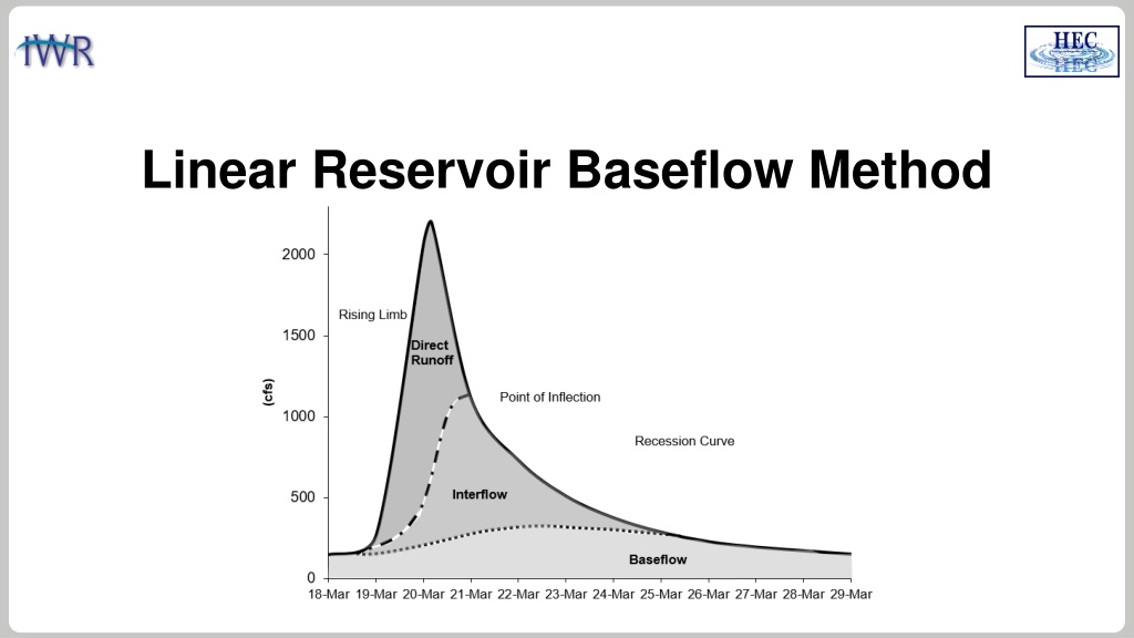
The linear reservoir baseflow method utilizes linear reservoirs to simulate the movement of water infiltrated into the soil. This method models water movement from the land surface to the stream network by integrating a linear relationship between storage and discharge. Users can select from one, two, or three linear reservoir layers, each with adjustable parameters such as initial discharge, fraction, linear reservoir coefficient, and number of steps. This approach is versatile, accommodating various loss methods and can help in analyzing baseflow contributions effectively.

Download Presentation

Please find below an Image/Link to download the presentation.
The content on the website is provided AS IS for your information and personal use only. It may not be sold, licensed, or shared on other websites without obtaining consent from the author. Download presentation by click this link. If you encounter any issues during the download, it is possible that the publisher has removed the file from their server.
E N D
Presentation Transcript
LINEAR RESERVOIR BASEFLOW The linear reservoir baseflow method uses linear reservoirs to model the movement of infiltrated water through the soil, and back onto the land surface and through the stream network. The continuity equation is used along with a linear relationship between storage and discharge: Interflow - Linear Reservoir Baseflow - Linear Reservoir dS/dt = change in storage at time t It= average inflow to storage at time t Ot= outflow from storage at time t R = linear reservoir coefficient 2
LINEAR RESERVOIR BASEFLOW The linear reservoir baseflow method is designed to work with all loss methods. Canopy Linear reservoir baseflow is explicitly identified in the Soil Moisture Accounting loss method. Surface All losses in the Initial and Constant, Curve Number, and Green and Ampt loss methods are available to the Linear Reservoir Baseflow (can overcome this assumption using the fraction option). Moisture Deficit Deficit/Constant Linear Reservoir Baseflow Constant Loss Rate Layer 1 Only constant loss rate losses (represents saturated conditions) in the Deficit and Constant loss method is available to the Linear Reservoir Baseflow. Layer 2 Layer 3 3
LINEAR RESERVOIR BASEFLOW You can choose 1, 2, or 3 linear reservoir layers. Each layer requires an initial discharge, fraction, linear reservoir coefficient, and number of steps. The fractions do not have to sum to 1. If they do not, the remainder represents water percolating to a deep aquifer. Canopy Surface Moisture Deficit Deficit/Constant Linear Reservoir Baseflow Constant Loss Rate Layer 1 Layer 2 Layer 3 4
LINEAR RESERVOIR BASEFLOW The example on this slide shows two linear reservoir layers. 40 percent of the infiltrated water is routed within Layer 1. 60 percent of the infiltrated water is routed within Layer 2. Notice the linear reservoir coefficients are different. Groundwater 1 can be used to model interflow, and groundwater 2 can be used to model groundwater flow. Canopy Surface Moisture Deficit Deficit/Constant Linear Reservoir Baseflow Constant Loss Rate Layer 1 Layer 2 Layer 3 5
LINEAR RESERVOIR BASEFLOW The plot on this slide shows three different simulations with different linear reservoir coefficients. Notice how larger coefficient values attenuate the baseflow contribution, which reflects longer durations the infiltrated water spends in the ground. Total Flow Coef. = 12 hours Coef. = 24 hours Coef. = 48 hours Notice that the timing of the baseflow hydrograph is not influenced much by the storage coefficient. Baseflow Initially set the coefficients using multipliers of the Clark Storage Coefficient. 6
LINEAR RESERVOIR BASEFLOW The plot on this slide shows three different simulations where the number of steps was varied. 2 steps means water flows into one linear reservoir with a coefficient of 24 hours, and then water from the first linear reservoir is routed through a second linear reservoir that also has a coefficient of 24 hours. Total Flow Steps = 1 Steps = 2 Steps = 3 Baseflow Notice how timing of the baseflow hydrograph is shifted and attenuation is increased as the number of linear reservoirs is increased. 7
LINEAR RESERVOIR BASEFLOW The plot on this slide shows three different simulations where the groundwater 2 linear reservoir coefficient was varied (50-50 split in infiltrated losses between layers). Groundwater 2/3 layers can be used to model the longer responding groundwater flow, these components will not have as much of an impact on the flood magnitude. Total Flow GW2 Coef. = 100 hours GW2 Coef. = 200 hours GW2 Coef. = 300 hours Baseflow 8
LINEAR RESERVOIR BASEFLOW The plot on this slide shows three different simulations where the groundwater fraction was varied. The fraction can be used to control the magnitude of the baseflow hydrograph (emphasize interflow), the fraction can be used to improve runoff volume. Total Flow GW 1 Fraction = 1 (volume 1.6 inches) GW 1 Fraction = 0.5 (volume 0.8 inches) GW 1 Fraction = 0.1 (volume 0.2 inches) Baseflow 9
LINEAR RESERVOIR BASEFLOW You can choose an initial discharge type: Discharge per Area or Discharge (a discharge per area of 1 CFS/MI2 means the initial flow would be 100 cfs for a 100 square mile subbasin) Discharge per Area is easier to apply across the basin model (generally consistent across subbasins), where a discharge initial type is dependent on the subbasin size. The plot on this slide shows different initial discharge per area values, manually adjust the initial discharge to match observations at the beginning of the simulation. Be strategic when setting the starting date of the simulation, interflow could be set to zero and only initial GW2/3 specified. Initial GW2 Disch. = 1 CFS/MI2 Initial GW2 Disch. = 5 CFS/MI2 Initial GW2 Disch. = 10 CFS/MI2 10
LINEAR RESERVOIR BASEFLOW Computed Total Flow Computed Baseflow Observed Flow The linear reservoir baseflow method can be used for a continuous simulation. The plot on this slide also shows that the linear reservoir method can simulate both interflow and groundwater flow (because it includes up to three layers, each layer has its own coefficient). 11