Understanding Linear Programming: An Introduction to Optimization
Linear programming, introduced by mathematician George B. Dantzig in 1947, is a mathematical technique for optimizing resource allocation in a systematic manner. It involves formulating linear relationships among variables to achieve desired results like cost minimization or profit maximization. Linear programming helps in determining rational proportions of inputs for achieving optimal outcomes in various real-world applications. This article provides insights into the definitions of linear programming, types of problems it can solve, and its classifications into general and duality problems.
Download Presentation

Please find below an Image/Link to download the presentation.
The content on the website is provided AS IS for your information and personal use only. It may not be sold, licensed, or shared on other websites without obtaining consent from the author. Download presentation by click this link. If you encounter any issues during the download, it is possible that the publisher has removed the file from their server.
E N D
Presentation Transcript
Introduction Introduced Mathematician George B. Dantzig in 1947 by a Russian
Introduction The name Linear Programming consists of the two important terms Programming. The term Linear refers to the relationship of the interrelated variables which is of the form of y = a + bx where x and y are the variables of power one and a and b are constants. viz., Linear and
Introduction The term programming means planning a way of action in a systematic manner with a view to achieving some desired optimal results, viz., the minimization of cost, maximization of profit etc.
Introduction Thus Linear Programming is a Mathematical technique which is applied in the form of a linear formula for arriving at a rational proportion of the variables to be used as inputs to get the optimum result from a course of action to be planned accordingly.
Definitions (LPP) According to Dantzig Linear Programming is defined as A programming of interdependent activities in a linear structure . According to Galton, Linear Programming is a mathematical technique for determining the optimal solution of resources and obtaining a particular objective where there are alternative uses of resources, viz., man material, machinery and money etc .
Definitions (LPP) From the above definitions it will be clear that linear programming is a mathematical device of ascertaining the optimal allocation of resources for obtaining the desired objective, viz., maximization of profit, or minimization of cost where various resources can be used alternatively.
Types of Problems (where L.P. can be applied) (1) Problems of allocation (2) Problems of assignment, and (3) Problems of transportation.
TYPES OF LINEAR PROGRAMMING PROBLEMS Linear Programming problems are classified into two types. They are (1) General or Primal linear programming problem (2) Duality linear programming problem.
General or Primal Linear Programming Problem Determination of the desired results under this type of problem will involve the following steps: Step No. 1. Formulation of the Given Problem Step No. 2. Solution of the Formulated Problem Each of the above steps will again require the following sub steps.
Formulation of L.P. Problem Under this step (i) Objective function (Z) (ii) Constraint functions, and (iii) Non negative functions.
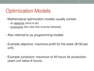
Objective Function The objective of a problem may be either to maximize or minimize some result. If it is a case of profit or income or output the objective must be maximization. But if it is a case of loss, cost or input, the objective will be minimization. For this the rate of profit or cost per variable in issue must be assessed first and then the number of each variable will be represented in the function through some letters viz. (namely) x, y to be ascertained through the process of solution. As such the objective function will be presented in the following form: Z(p) = P1X1 + P2X2 + ......+PnXn ( Z=3X1+4X2) where, Z(p) = Maximum amount of profit Variables x and y are called decision variables.
Objective Function P1, P2, ..., Pn = Rate of profit per different variables to be produced, viz., goods or services X1, X2, ..., Xn = The number of different variables to be produced under decision.
Objective Function In case of variables involving cost or loss the objective will be minimization and in that case the objective function will be formulated as under: Z(c) = C1X1 + C2X2 + ......+CnXn (Z = 3X1+4X2) where, Z(c) = Minimum amount of cost C1, C2, ..., Cn = Cost per unit of the variable. X1, X2, ..., Xn = Different number of the different variable..
Constraint Function To accomplish the desirable objective it is necessary to put some resources, viz., manpower, material, machine or money in the process of production or performance. But such resources may not be available in unlimited quantity in all the cases. There are some resources which may be available to a limited extent and thus create constraints or bottlenecks in the process of performance. There are also some resources whose availability cannot be obtained below a certain extent and thus compels the management to procure them in certain larger quantities. However, there might be some resources, which may be available to the extent just required for the purpose.
Constraint Function These resources, therefore, do not create any obstacle. But the resources which are available up to or beyond certain limit create constraints in achieving the objective. Thus the objective function will be adjusted in the light of the given constraints relating to the availability of the various resources. Thus, the objective function will be follows by the constraint functions in the following manner.
Constraint Function The restrictions on the variables of a linear programming problem are called constraints. The conditions x 0, y 0 are called non- negative restrictions. In the next slide, the set of inequalities (1) to (3) are constraints. linear inequalities or equations or
Constraint Function Process I : a11X1 + a12X2 + ... + a1nXn b1 Process II : a21X1 + a22X2 + ... + a2nXn b2 Process III : a31X1 + a32X2 + ... + a3nXn = b3
Non Negative Function This function implies that the production or performance of the variables in issue will never be negative. It will be either zero or greater than zero but never but never less than zero. This function is therefore represented as under: X1 0, X2 0, ..., Xn Thus the formulation phase of a primal linear programming problem will be constituted as below:
Non Negative Function Thus, a Linear Programming Problem is one that is concerned with finding the optimal value (maximum or minimum value) of a linear function (called objective function) of several variables (say x and y), subject to the conditions that the variables are non-negative and satisfy a set of linear inequalities (called linear constraints). The term linear implies that all the mathematical relations used in the problem are linear relations while the term programming refers to the method of determining a particular programme or plan of action.
Non Negative Function Optimisation problem A problem which seeks to maximise or minimise a linear function (say of two variables x and y) subject to certain constraints as determined by a set of linear inequalities is called an optimisation problem. Linear programming problems are special type of optimisation problems. The above problem of investing a given sum by the dealer in purchasing chairs and tables is an example of an optimisation problem as well as of a linear programming problem.
Formulation of L.P.P. (Primal) Maximize or Minimize Z = C1X1 + C2X2 + ..., CnXn Subject to constraint a11X1 + a12X2 + ... + a1nXn b1 a21X1 + a22X2 + ... + a2nXn b2 a31X1 + a32X2 + ... + a3nXn = b3 Subject to non-negativity condition that X1 0, X2 0, ..., Xn 0.
Feasible Region The set of all points satisfying all the LP's constraints.
Optimal Solution for a Maximization Problem: A point in the feasible region with the largest objective function value. Z= 3X+ 4Y
Optimal Solution for a Minimization Problem A point in the feasible region with the smallest objective function value. Z= 3X+ 4Y
Infeasible Solution A solution for which at least one constraint is violated.
Feasible Solution a solution for which all of the constraints are satisfied
Proportionality The basic assumption underlying the linear programming is that any change in the constraint inequalities will have the proportional change in the objective function. eg if production of one unit of a product uses 5 hours of a particular resource, then making 3 units of that product uses 3 X 5 = 15 hours of that resource
Additivity The assumption of additivity asserts that the total profit of the objective function is determined by the sum of profit contributed by each product separately. Similarly, the total amount of resources used is determined by the sum of resources used by each product separately.
Continuity Another assumption of linear programming is that the decision variables are continuous. This means a combination of outputs can be used with the fractional values along with the integer values.
Certainty Another underlying assumption of linear programming is a parameters of objective function coefficients and the coefficients of constraint inequalities is known with certainty. Such as profit per unit of product, availability of material and labor per unit, requirement of material and labor per unit are known and is given in the linear programming problem. certainty, i.e. the
Finite Choices This assumption implies that the decision maker has certain choices, and the decision variables assume non-negative values. The non-negative assumption is true in the sense, the output in the production problem can not be negative. Thus, this assumption is considered feasible.
Finite Choices 1. LP makes logical thinking and provides better insight into business problems. 2. Manager can select the best solution with the help of LP by evaluating the cost and profit of various alternatives. 3. LP provides an information base for optimum allocation of scarce resources.
Finite Choices 4. LP assists in making adjustments according to changing conditions. 5. LP helps in solving multi-dimensional problems.
Limitations 1. This technique could not solve the problems in which variables cannot be stated quantitatively. 2. LP technique cannot solve the business problems of non- linear nature. 3. The factor of uncertainty is not considered in this technique. 4. This technique is highly mathematical and complicated. 5. If the numbers of variables or constrains involved in LP problems are quite large, then using costly electronic computers become essential, which can be operated, only by trained personnel. 6. Under this technique to explain clearly the objective function is difficult.
Managerial uses and Applications (a) Optimizing the product mix when the production line works specification; (b) Securing least cost combination of inputs; (c) Selecting the location of Plant; (d) Deciding the transportation route; (e) Utilizing the storage and distribution centres under certain
Managerial uses and applications (f) Proper production scheduling and inventory control (g) Minimizing the raw materials waste (h) Assigning job to specialized personnel.
Optimal (feasible) solution Any point in the feasible region that gives the optimal value (maximum or minimum) of the objective function is called an optimal solution
Duality in Linear Programming Definition: Programming programming problem has another linear programming problem related to it and thus can be derived from it. The original linear programming called Primal, while the derived linear problem is called Dual. The states Duality that in Linear linear every problem is
Duality in Linear Programming Before solving for the duality, the original linear programming problem is to be formulated in its standard form. Standard form means, all the variables in the problem should be non-negative and , sign is used in the minimization case and the maximization case respectively. The concept of Duality can be well understood through a problem given below:
Formulating a Dual Problem Steps for formulation are summarised as Step 1: write the given LPP in its standard form. 2: identify the variables of dual problem which are same as the number of constraints equation. 3: write the objective function of the dual problem by using the constants of the right had side of the constraints. Step 4: if primal is max/min type than dual is min/max type and the constraints are / type. Step 5: dual variables are unrestricted in sign.
Maximization Problem Primal
Duality in Linear Programming The primal or original linear programming problem is of the maximization type while the dual problem is of minimization type. The constraint values 100 and 150 of the primal problem have become the coefficient of dual variables y1and y2in the objective function of a dual problem and while the coefficient of the variables in the objective function of a primal problem has become the constraint value in the dual problem.
Duality in Linear Programming The first column in the constraint inequality of primal problem has become the first row in a dual problem and similarly the second column of constraint has become the second row in the dual problem. The directions of inequalities have also changed, i.e. in the dual problem, the sign is the reverse of a primal problem. Such that in the primal problem, the inequality sign was but in the dual problem, the sign of inequality becomes .
The dual of a dual problem is the primal problem.
Rules for Constructing the Dual from Primal
Rules for Constructing the Dual from Primal 1. A dual variable is defined corresponds to each constraint in the primal LP problem and vice versa. Thus, for a primal LP problem with m constraints and n variables, there exists a dual LP problem with m variables and n constraints and vice-versa. 2. The right-hand side constants b1, b2, . . ., bm of the primal LP problem becomes the coefficients of the dual variables y1, y2, . . ., ym in the dual objective function Zy. Also the coefficients c1, c2, . . ., cn of the primal variables x1, x2, . . ., xn in the objective function become the right-hand side constants in the dual LP problem.
Rules for Constructing the Dual from Primal 3. For a maximization primal LP problem with all (less than or equal to) type constraints, there exists a minimization dual LP problem with all (greater than or equal to) type constraints and vice versa. Thus, the inequality sign is reversed in all the constraints except the non-negativity conditions. 4. The matrix of the coefficients of variables in the constraints of dual is the transpose of the matrix of coefficients of variables in the constraints of primal and vice versa.
Rules for Constructing the Dual from Primal 5. If the objective function of a primal LP problem is to be maximized, the objective function of the dual is to be minimized and vice versa. 6. If the ith primal constraint is = (equality) type, then the ith dual variables is unrestricted in sign and vice versa
