Understanding Ordinary Differential Equations (ODEs) in Mathematics
Ordinary Differential Equations (ODEs) play a crucial role in modeling various physical phenomena and engineering problems. This lecture delves into the basics of ODEs, discussing their applications, solution methods, and interpretation in real-world scenarios. Mathematical modeling is highlighted as a key process in translating physical situations into mathematical models for analysis and prediction.

Download Presentation

Please find below an Image/Link to download the presentation.
The content on the website is provided AS IS for your information and personal use only. It may not be sold, licensed, or shared on other websites without obtaining consent from the author. Download presentation by click this link. If you encounter any issues during the download, it is possible that the publisher has removed the file from their server.
E N D
Presentation Transcript
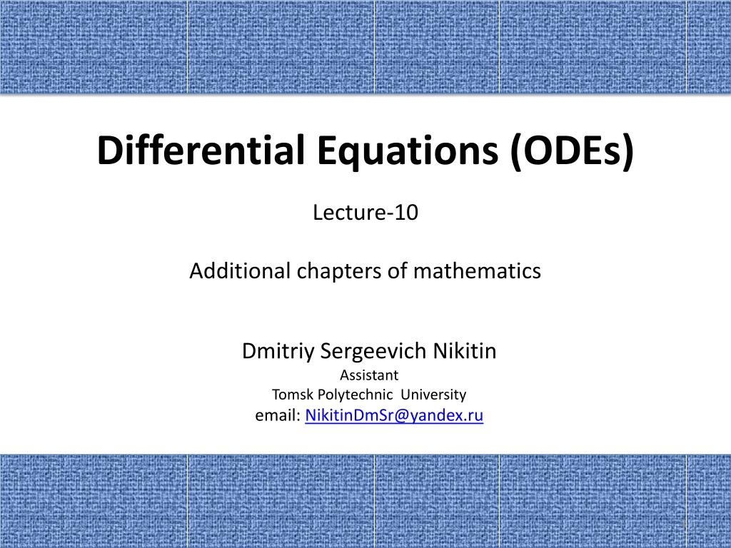
Differential Equations (ODEs) Lecture-10 Additional chapters of mathematics Dmitriy Sergeevich Nikitin Assistant Tomsk Polytechnic University email: NikitinDmSr@yandex.ru 1
Ordinary Differential Equations (ODEs) Many physical laws and relations can be expressed mathematically in the form of differential equations. Indeed, many engineering problems appear as differential equations. Ordinary differential equations (ODEs) are differential equations that depend on a single variable. The more difficult study is associated with partial differential equations (PDEs) that depend on several variables. 2
Ordinary Differential Equations (ODEs) Modelingis a crucial general process in engineering, physics, computer science, biology, medicine, environmental science, chemistry, economics, and other fields that translates a physical situation or some other observations into a mathematical model. Numerous examples from engineering (e.g., mixing problem), physics (e.g., Newton s law of cooling), biology (e.g., Gompertz model), chemistry (e.g., radiocarbon dating), environmental science (e.g., population control) are explained in terms of differential equations. 3
Ordinary Differential Equations (ODEs) This lecture begins the study of ordinary differential equations (ODEs) by deriving them from physical or other problems (modeling), solving them by standard mathematical methods, and interpreting solutions and their graphs in terms of a given problem. The simplest ODEs to be discussed are ODEs of the first order because they involve only the first derivative of the unknown function and no higher derivatives. These unknown functions will usually be denoted by y(x) or y(t) when the independent variable denotes time t. Understanding the basics of ODEs requires solving problems by hand (paper and pencil, or typing on your computer, but first without the aid of a CAS Computer Algebra System). 4
Mathematical modeling If we want to solve an engineering problem (usually of a physical nature), we first have to formulate the problem as a mathematical expression in terms of variables, functions, and equations. Such an expression is known as a mathematical model of the given problem. The process of setting up a model, solving it mathematically, and interpreting the result in physical or other terms is called mathematical modeling or, briefly, modeling. Modeling needs experience, which we will gain by discussing various examples and problems (your computer may often help you in solving but rarely in setting up models). 5
Mathematical modeling Now many physical concepts, such as velocity and acceleration, are derivatives. Hence a model is very often an equation containing derivatives of an unknown function. Such a model is called a differential equation. Of course, we then want to find a solution (a function that satisfies the equation), explore its properties, graph it, find values of it, and interpret it in physical terms so that we can understand the behavior of the physical system in our given problem. However, before we can turn to methods of solution, we must first define some basic concepts. 6
Differential equations An ordinary differential equation (ODE) is an equation that contains one or several derivatives of an unknown function, which we usually call y(x) (or sometimes y(t) if the independent variable is time t). The equation may also contain yitself, known functions of x(or t), and constants. For example, ? = ????or? + ?? = ? ??are ordinary differential equations (ODEs). Here, as in calculus, ? denotes ??/??, ? = ???/??? etc. The term ordinary distinguishes them from partial differential equations (PDEs), which involve partial derivatives of an unknown function of two or more variables. For instance, a PDE with unknown function u of two variables x and y is ??? ???+??? ???= ? 8
First-order ODEs An ODE is said to be of order nif the n-th derivative of the unknown function yis the highest derivative of yin the equation. The concept of order gives a useful classification into ODEs of first order, second order, and so on. We will consider first-order ODEs. Such equations contain only the first derivative ? and may contain y and any given functions of x. Hence we can write them as ?(?,?,? ) = ? (1) or often in the form ? = ? ?,? . This is called the explicit form, in contrast to the implicit form(1). 9
Concept of Solution A function ? = ? ? is called a solution of a given ODE (1) on some open interval ? < ? < ? if ? ? is defined and differentiable throughout the interval and is such that the equation becomes an identity if y and ? are replaced with h and? , respectively. The curve (the graph) of h is called a solution curve. Here, open interval ? < ? < ? means that the endpoints a and b are not regarded as points belonging to the interval. Also, ? < ? < ? includes infinite intervals < ? < ?, ? < ? < , < ? < (the real line) as special cases. 10
Concept of Solution Each ODE has a solution that contains an arbitrary constant c. Such a solution containing an arbitrary constant cis called a general solution of the ODE (we will see that cis sometimes not completely arbitrary but must be restricted to some interval to avoid complex expressions in the solution). We will develop methods that will give general solutions uniquely. Hence we will say thegeneral solution of a given ODE (instead of ageneral solution). Geometrically, the general solution of an ODE is a family of infinitely many solution curves, one for each value of the constant c. If we choose a specific cwe obtain what is called a particular solution of the ODE. A particular solution does not contain any arbitrary constants. In most cases, general solutions exist, and every solution not containing an arbitrary constant is obtained as a particular solution by assigning a suitable value to c. 11
Concept of Solution In most cases the unique solution of a given problem, hence a particular solution, is obtained from a general solution by an initial condition ? ?? = ??, with given values ?? and ??, that is used to determine a value of the arbitrary constant c. Geometrically this condition means that the solution curve should pass through the point (??,??) in the xy-plane. An ODE, together with an initial condition, is called an initial value problem. Thus, if the ODE is explicit, ? = ? ?,? , the initial value problem is of the form ? = ? ?,? ? ?? = ?? (2) 12
More on Modeling We will now consider a basic physical problem that will show the details of the typical steps of modeling. Step 1: the transition from the physical situation (the physical system) to its mathematical formulation (its mathematical model); Step 2: the solution by a mathematical method; Step 3: the physical interpretation of the result. This may be the easiest way to obtain a first idea of the nature and purpose of differential equations and their applications. Realize at the outset that your computer (your CAS) may perhaps give you a hand in Step 2, but Steps 1 and 3 are basically your work. And Step 2 requires a solid knowledge and good understanding of solution methods available to you you have to choose the method for your work by hand or by the computer. 13
Complex Form of the Fourier Integral A first-order ODE (1) ? = ? ?,? (3) has a simple geometric interpretation. From calculus you know that the derivative ? (?) of ?(?) is the slope of ?(?). Hence a solution curve of (3) that passes through a point (??,??) must have, at that point, the slope ? ?? equal to the value of f at that point; that is, ? ?? = ? ??,??. Using this fact, we can develop graphic or numeric methods for obtaining approximate solutions of ODEs (3). This will lead to a better conceptual understanding of an ODE (3). Moreover, such methods are of practical importance since many ODEs have complicated solution formulas or no solution formulas at all, whereby numeric methods are needed. 14
Graphic Method of Direction Fields Practical Example Illustrated in Figure. We can show directions of solution curves of a given ODE (3) by drawing short straight- line segments (lineal elements) in the xy- plane. This gives a direction field (or slope field) into which you can then fit (approximate) solution curves. This may reveal typical properties of the whole family of solutions. Figure shows a direction field for the ODE ? = ? + ? (2) obtained by a CAS (Computer Algebra System) and some approximate solution curves fitted in. 15
Separable ODEs Many practically useful ODEs can be reduced to the form ?(?)? = ? ? by purely algebraic manipulations. Then we can integrate on both sides with respect to x, obtaining ?(?)? ?? = ? ? ?? + ? (5) On the left we can switch to y as the variable of integration. By calculus, ? ?? = ??, so that ?(?) ?? = ? ? ?? + ? (6) If f and g are continuous functions, the integrals in (6) exist, and by evaluating them we obtain a general solution of (4). This method of solving ODEs is called the method of separating variables, and (4) is called a separable equation, because in (6) the variables are now separated: x appears only on the right and y only on the left. (4) 16
Extended Method: Reduction to Separable Form Certain nonseparable ODEs can be made separable by transformations that introduce for y a new unknown function. We discuss this technique for a class of ODEs of practical importance, namely, for equations ? = ? ? ?. ?, such as sin ? (7) ? Here, f is any (differentiable) function of ? and so on. Such an ODE is called a homogeneous ODE. The form of such an ODE suggests that we set ? ? = ?? and by product differentiation ? = ? ? + ? (8) Substitution into ? =? ? ? = ? ? ?. We see that if ? ? ? ?, this can be ?? ? ? ?=?? ? ? ?, ?= ?; thus, ? ? then gives ? ? + ? = ?(?) or ?. (9) separated: 17
Linear ODEs Linear ODEs or ODEs that can be transformed to linear form are models of various phenomena, for instance, in physics, biology, population dynamics, and ecology. A first-order ODE is said to be linear if it can be brought into the form ? + ? ? ? = ? ? . (10) by algebra, and nonlinear if it cannot be brought into this form. The defining feature of the linear ODE (10) is that it is linear in both the unknown function y and its derivative ? = ??/?? whereas p and r may be any given functions of x. If in an application the independent variable is time, we write t instead of x. If the first term is ?(?)? (instead of ? ), divide the equation by ?(?) to get the standard form (10), with ? as the first term, which is practical. For instance, ? ??? ? + ? ??? ? = ? is a linear ODE, and its standard form is ? + ? ?? ? = ? ??? ?. The function r(x) on the right may be a force, and the solution y(x) a displacement in a motion or an electrical current or some other physical quantity. In engineering, is frequently called the input, and y(x) is called the output or the response to the input (and, if given, to the initial condition). 18
")
")
")
")