Understanding Differential Equations in Economics Honours

Differential equations, introduced by Newton and Leibniz in the 17th century, play a key role in economics. These equations involve derivatives and represent implicit functional relationships between variables and their differentials, often related to time functions. The order and degree of a differential equation determine its complexity. There are different types of differential equations, including ordinary and partial types. Solutions to these equations involve general solutions with arbitrary constants that can be narrowed down to particular solutions by assigning specific values based on initial conditions. One specific type discussed is the first-order linear differential equation with constant coefficients and terms.

Download Presentation

Please find below an Image/Link to download the presentation.
The content on the website is provided AS IS for your information and personal use only. It may not be sold, licensed, or shared on other websites without obtaining consent from the author. Download presentation by click this link. If you encounter any issues during the download, it is possible that the publisher has removed the file from their server.
E N D
Presentation Transcript
DIFFERENTIAL EQUATIONS SEM 3 ECONOMICS HONOURS
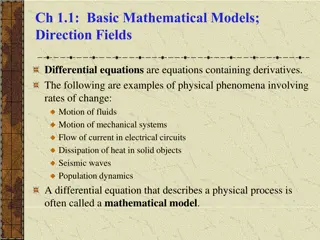
Differential Equations Differential Equations were begun by Newton and Leibniz in the seventeenth century. Differential Equations are often used in economics. A Differential Equation is an equation which involves derivatives. It is an implicit functional relationship between variables and their differentials. The unknown is often a function of time.
Order and degree of Differential Equations The order of a Differential Equation is the highest order of any of the derivatives contained in it. A Differential Equation is of order n if the nth derivative is the highest order derivative in it. The highest power to which the derivative of the highest order occur is the degree of a Differential Equation.
Example of Differential Equation Y = dy/dt + t2 Differential Equation of order 1 and degree 1 (d2y/dt2)3 6 (dy/dt)2+ty = 0 Differential Equation of order 2 and degree 3
Kinds of Differential Equations Ordinary Type: involving only one independent variable and its derivatives. Partial Differential Equations: involving more than one independent variable and partial derivatives.
Solution of Differential Equation Differential Equation of order n has a General solution containing n arbitrary independent constants. A Particular solution may be obtained from the general solution by assigning certain specific values [which are obtained from any given information of the initial conditions given in the problem] to the arbitrary constants .
First- order linear Differential Equation with constant coefficient and constant term General form of the equation: dy/dt + u(t) y = w(t) derivative is taken with respect to time (t) u and w are functions of t When u and w are taken as constant, the is termed as First- order linear Differential Equation with constant coefficient and constant term.
Homogeneous Case U = a constant ; a W = 0 the form of the Equation becomes : dy/dt + ay = 0 => 1/y dy/dt = -a => 1/y dy = - a dt [taking integration of both side] 1 From left side, 1/y dy = log y + c1(y#0) From right side, - a dt = -at + c2 By equating, log y = -at + c
Now taking anti log of log y implies, elog y = x therefore, , log y = -at + c becomes, elog y = e-at + c=> y = e-at . ec= A. e-at Therefore the solution is y(t) = A. e-at 2 This is general solution, where A is arbitrary. For any particular value of A the solution becomes particular. There may be infinite number of particular solution. Setting t=o , y(0) = A . e0=> A = Y (0) Therefore Y(t) = Y(0)e-at .. 3 This is the Definite Solution as the arbitrary constant is definitized here. Y(0) is the only value that makes the solution satisfy the initial condition.
Note: The solution is a function of Y(t) a time path where t symbolizes time. No derivative is present in the solution.
The Non-homogeneous Case The equation is dY/dt + aY = b ....... 4 The solution is the sum of Complementary function and Particular Integral. To find Particular integral ( Yp) , y is taken as a constant. Here Y = k , dY/dt = 0 Equation 4 becomes, ak = b => k = b/a = Yp... 5a
To get the Complementary Function (Yc), the process is to get the homogeneous equation which is termed as reduced equation. The Trial solution is Yc= A e at....5b So, the general solution becomes Y(t) = Yc+ Yp= A e at+ b/a ........6 .
Now the constant A is definitized by means of an initial condition. When t = 0 , y takes the value Y(0) . Equation 6 becomes, Y(0) = A + b/a => A = Y(0) - b/a Therefore the definite solition is Y(t) = [ Y(0) b/a] e-at+ b/a ........7
Use of Differential Equation in Economics Differential Equations have wide use to explain different concepts of Economics. Equilibrium, Stability of different Market models can be easily explained by this mathematical method. Growth models also use linear differential Equation.
Analysis of Equilibrium is an important part of Economics. Differential Equations explains the Euilibrium as well as the investigates the Stability of Equilibrium. In the above discussed linear differential equation, the time path of Y is obtained. The solution is given here once more: Y(t) = [ Y(0) b/a] e-at+ b/a ............ 7 Equilibrium can be attained if , Y(0) = b/a When Y(0) b/a , it requires to analyse whether the time path converges to equilibrium over time or not and this is called the Stability Analysis. The stability depends on the value of a . From equation 7 it can be shown that, starting from a non-equilibrium position, Convergence is obtained if e-at 0 as t It is possible only when a > 0 Divergence is obtained e-at as t It is possible only when a < 0


, the process is")