Equations of State in Thermodynamics
In the study of thermodynamics, equations of state play a crucial role in predicting the behavior of substances based on pressure, volume, and temperature relationships. These equations define the interdependence of various intensive properties for a simple compressible substance. The development and characteristics of PvT models are discussed, along with the considerations for accuracy, precision, and input data requirements in creating these equations. The critical behaviors and isometric lines on the PT diagram are also explored.

Download Presentation
Please find below an Image/Link to download the presentation.
The content on the website is provided AS IS for your information and personal use only. It may not be sold, licensed, or shared on other websites without obtaining consent from the author. Download presentation by click this link. If you encounter any issues during the download, it is possible that the publisher has removed the file from their server.
Presentation Transcript
Chapter Five Equation of state 1
5.1 INTRODUCTION State postulate of a simple compressible substance: any intensive property is solely a function of two other independent, intensive properties. The ones that relate P, v, and T are usually known as equations of state whose functional form looks like f(P,v,T)=0 (algebraic equation, graph or a set of tabular data) Initially discussions will be on algebraic ones. 2
An equation of state serves two purposes: Prediction of PvT behavior of substances; uses PvT cartesian coordinates ; Pv plane is a typical case usually represented on reduced pressure (Pr), reduced temperature (Tr) and reduced specific volume (vr) coordinate systems. Typical Pv surface is shown in Fig 5.1 P v T P v T r r r P v T c c c For large values of vr fairly simple mathematical expression can be used to represent an isotherm with reasonable accuracy. 3
Fig.5.1 Experimental Pr - vr relationships for argon along isotherms Tr. 4
For low values of specific volumes (vr1) pressure changes rapidly for small changes in density-will require complex analytical solution. More complication is in the saturation region a region of discontinuity. The other major use is in the evaluation of property data that can not be measured directly; u, h, s, cp, cv, g, a, and f. Usually the mathematical relationships for these properties contain first and second derivatives. Such a function must lend itself to differentiation and integration. In addition the functions must exhibit some unique PvT characteristics experienced by all substances 5
Three primary decisions to be made in the development of equation of state: range of values of interest (density);precision or accuracy; amount and kind of input data 5.2 CHARACTERISTIC OF PvT BEHAVIOR Some criteria which the PvT models should fulfill: At the critical point, the critical isotherm has an inflection and horizontal slope, requiring c T v 2 P P = = 0 0 and 2 v which must be fulfilled by the model function T c 6
All isometric lines on the PT diagram are nearly straight (linear). In particular, the slope of the critical isometric is equal to the slope of the vapor pressure curve. So the model must meet this requirement Fig 5.2. Replotting the vapor pressure curve as log10 Pr versus 1/Tr, experimental data indicate that the lines are nearly straight. 2 d (log P ) 1 d ln P 1 T dP = = = = 10 T r r r r / 1 ( d ) . 2 303 / 1 ( d T . 2 303 P dT r r r r This can be seen to be directly related (dP/dT)crit as follows: 7
Fig.5.2 PT diagram showing the vapor-pressure curve for a pure substance and constant-volume lines in the single-phase regions 8
At the critical state Tr=1 and Pr=1. The above equation will give dP T d crit r r 303 . 2 ) / 1 ( dP (log10 ) 1 d P T = = . 0 = . 0 434 434 r c r m dT P dT c crit where dP T dP = det min c r m er ed by the unique dT P dT r c crit crit derivative at the critical state The value of m determined from vapor pressure data derivative at the critical point must match that obtained from the model equation. The lines in Fig 5.3 represent various values of m. 9
Fig.5.3 Generalized vapor-pressure plot Example 5.1 (a) Estimate constants A and B in the linear vapor-pressure equation log10??= ? + steam, using data at the critical state and another saturation state near the critical state. (b) Estimate the value of m for steam . ? ??for
Other general PvT characteristics gases exhibit are 1. As P approaches zero, gases behave as ideal gases and RT Pv = = lim lim 1 Z P 0 0 P 2.Also as P approaches zero videal-vactual is a non-zero value known as residual volume which is solely a function of temperature. The model should predict with a reasonable accuracy (Fig 5.4) RT P = = lim0 ( ) v f T P 3. Critical isotherm essentially vertical at high pressures, ie. V is constant at the critical temperature and high pressure as given by Redlich-Kwong equation was devised empirically to satisfy this criterion. lim ( ) . 0 26 v v P T c c 11
Fig.5.4 Isotherms for the residual volume versus pressure for CO and CO2. 12
4. Range of Zc for any substance is between 0.22 and 0.30. Therefore for all gases the model must predict (for all gases) P v = 3 . 0 . 0 22 c c Z c RT c 5. The critical isometric line (straight line) on a PT diagram must satisfy (in the super heat region) c v Although it would be difficult to satisfy all these and other additional criteria it would be hoped that any equation of state would reproduce a number of these characteristics with reasonable accuracy. 2 P = 0 2 T 13
The following is a review of some of the more important equations of state. 5.3 THE COMPRESSIBILITY FACTOR The equation Pv=ZRT predicts the real gas behavior where Z is known as the compressibility factor, indicator of the degree of deviation from ideal gas behavior. Also Z=(vact/videal) 14 Fig.5.5 Compressibility plot for nitrogen gas
5.4 TWO-PARAMETER CUBIC EQUATION OF STATE This is the simplest for predicting both vapor and liquid behavior. It is cubic in v. 5.4.1 van der Waals Equation It is the first equation, after J.D. van der Waals in 1873. Basis: Attractive forces reduce the pressure below Pideal (pressure correction is inversely proportional to v2)and particles have finite sizes and this reduces the volume available to the molecules. Thus 2 also v a RT a = = P P P act ideal 2 v b v 15
For the constants the critical isotherm at the critical state was considered. c T v 2 P P = = 0 0 and 2 v T c Differentiation will give = c T v v c 2 2 2 v 6 v RT RT P a P a + = = = 0 0 c c 3 4 2 2 3 ( ) ( ) b v v b c c c T c Two equations and two unknowns give 9 RT v v = = c c c a and b 8 3 Insertion into RT a = c P will give c 2 v b v 16 c c
3 3 RT P v = = = = . 0 375 c c c P gives Z c c 8 8 v RT c c (which is out of the range 0.22-0.30) The above equation will enable to express the constants in terms of vc and Pc or Tc and Pc. The latter is preferred. c b P 64 2 2 27 R T RT 8 = = c a P c c These values will be different from the previous values as the equation for Pc is not valid when actual data are used.High value of Zc leads to another problem. With reference to Fig 5.6 it may be shown that vdW c vdW c Z v , , Zc=0.291 will give vc,vdW=1.29vc,act v Z And applying on, for example, argon, = , , c act c act 17
vdW equation is good in predicting at low pressures. Fitting experimental PvT data can be used to determine the constants. In the absence of data the inflection points at the critical state are commonly used to evaluate a and b. Solutions of vdW equations on isotherms 1. T>Tc- two imaginary roots and one real positive root; pressure monotonically decreases with increase in v (Fig 5.7) 2. T=Tc-at critical pressure three real and equal roots 3. T<Tc-below Pc, three real and unequal roots 19
The vdW and any other cubic equation can be transformed into the form Z=f(Tr,Pr). In this case 2 27 27 P P P + = 3 2 0 r r r Z Z Z 2 3 8 T 64 512 T T r r r 5.4.2 Redlich-Kwong Equation (RK) Published in 1949, widely accepted cubic equation, considerably more accurate than vdW equation. a b v RT = P + / 1 2 ( ) T v v b Does quite well at small to moderate densities and is much better when T>Tc. If PvT data are not available the constants a and b can be determined using the inflection point on Tc at the critical point as: 21
5 . 2 c 5 . 2 c 2 2 R T R T R T R T = = = = = = = = a 42748 . 0 b 08664 . 0 c c a b P P P P c c c c P v 1 = = Z c c = = , c RK RT 3 c 2 P 5 . 2 r P P P + + + + = = 3 2 Z Z 1 Z 0 r r r r a b b a b 5 . 3 r T T T T r r When P and T are known, vdW and RK require solution of cubic equations in v. 22
5.5 THE CORRESPONDING STATES PRINCIPLE The functional relationship Z=f(Tr,Pr) is known as the vdW two-parameter theorem of corresponding states. Also known as generalized equation. It states that any pure gas at the same Tr and Pr should have the same Z. From vdW and RK equations, it follows that the application extends to both single phases ie. saturated liquid and saturated vapor states. Fig 5.8 shows this function for 10 common substances (deviation from mean isotherms<1%). Nelson-Obert chart (avg behavior of 30 substances) predicts Z within 5-6% except near critical states. 23
Fig.5.8 Experimental data correlation for a generalized Z chart.
Z for polar substances can deviate by as much as 15- 20 %. For H2, He, and neon redefine Pr and Tr as: and C P c + P T + = = P T r r T C c For P(atm), T(K) C=8. To introduce v in the generalized charts (Zc=0.22-0.3) P RT T RT Pv P v P v P ' = = = = = = = = Z v ( Z ) v r r c c r r r c r T T r vP c r r T ' = = = = v v Z Z c r r r c RT P The above is the pseudo reduced volume used in the Nelson-Obert chart. c r 25
5.5.1 Three-Parameter Corresponding States Principle Failure of the two parameter corresponding states principle to predict Z accurately except for small number of substances indicates one or more additional parameters are required if better accuracy is desired for a larger number of substances. Experimental data indicate that Z tend to fall into three rough classes depending on the structures of molecules, degree of sphericity :spherical with respect to geometry and force field , moderately non- spherical and extremely non-spherical. The two-parameter equation is good for spherical molecules. A third parameter will be required for the other molecules. 26
5.5.2 The critical compressibilit ( Zc) as a Third Parrameter Lydersen, Greenkorn, and Hougen presented separate Z-Tr-Pr charts or tables for particular values of Zc. Such a chart represent the relation Z=f(Tr,Pr,Zc). Resulted in a significant improvement of accuracy. 5.5.3 The Acentric Factor as the Third Parameter Heavier permanent gases argon, krypton, and xenon qualify as having spherical molecules. Gases such as CH4, CO, N2, H2S have structures close to the above gases. These are simple fluids . Moderately non- spherical are classified as normal fluids. The naming is after Pitzer. 27
The third parameter measures the deviation from simple fluid behavior ie. Nonsphericity or acentricity. One parameter which fits is the vapor pressure data on a reduced basis. For two parameter fluids there will be a single slope (true for simple fluids). The position of the reduced vapor pressure curve of a fluid relative to the position of a simple fluid is a sensitive property which could be the basis for the third parameter. Pitzer used this to define a third parameter, , the acentric factor as the difference between the value of log10Prsat for the fluid and that for a simple fluid at a fixed value of Trsat. m=5.4, at Trsat=0.7, log10Prsat =-1for simple fluids. 28
With this data as a convenient reference for a non- spherical fluid ( log 0 . 1 = sat ) rP 7 . 0 = 10 r T (gives zero for simple fluids) Example 5.2 Determine the value of for water based on the above equation. The three-parameter corresponding states principle of Pitzer states that ? = ? ??,??,? A linear correlation was developed as Z=Z(0) + Z(1) The first expression is for simple fluids while the second is the deviation from simple fluid. Lee-Kessler revised and extended the data of Pitzer and have generated useful tables for Z(0) and Z(1). 29
A relatively complicated reference fluid, octane with a compressibility factor Z(r) is used to determine the correction factor Z(1), assumed to be a linear weighted average value such that + = r Z Z Z where = + ) 0 ( ( ) ) 0 ( ) 0 ( ) 1 ( r Z Z Z Z Z Z ( ) ) 0 ( r = = ) 1 ( ( ) r . 0 3978 and ( ) r tables.docx Example 5.3 examples.docx 30
5.6 THREE-PARAMETER CUBIC EQUATIONS OF STATE 5.6.1 Redlich-Kwong-Soave Equation Soave s modification of RK equation of states given by: 2 + 2 42748 . 0 08664 . 0 R T RT RT a = = = c c P a b ( ) v b v v b P P c c 1 2 / 1 r 2 = + = . 1 + 2 1 ( S ) . 0 48 574 . 0 176 T S Used in the prediction of thermodynamic properties of refrigerants. 31
5.6.2 Peng-Robinson Equation RT a ) = P same as in RKS + + ( ( ) v b v v . 1 + b b v b = 2 37464 . 0 54226 . 0 26992 S 2 2 45724 . 0 07780 . 0 R T RT = = c c a b P P c c PR equation has about the same accuracy as the RKS equation in predicting Z and specific volumes. 32
5.6.3 Generalization of Equation of States The four cubic equations seen so far and others can be expressed by a general relation of the form RT P + + = ( )( ) v b v c v d Values of , b, c, and d are given in tables. It can also be converted into a general reduced equation of the form f(Z,Pr,Tr, )=0 33
Equation c d b Van der Waals 0 0 RT 8 2 2 27 R T c c 64 P P c c Redlich-Kwong b 0 08664 . 0 RT 5 . 2 c 42748 . 0 RT c P 5 . 0 P T c c 08664 . 0 RT 2 Soave b 0 2 42748 . 0 R T c c P P c c 07780 . 0 Peng-Robinson (1+ 2)b (1- 2)b RT 2 2 45724 . 0 R T c c P P c c 34
5.7 OTHER EQUATIONS OF STATE Cubic equations extremely useful for predicting vapor and liquid PvT data, vapor-pressure data, and vapor-liquid equilibria data. Accuracy limited by the use of only two or three adjustable parameters. For a better overall accuracy, equations of greater complexity are used. 5.7.1 Virial Equations Statistical mechanics reveals that a theoretical equation relating Z to PvT data should take the form of a series expansion in 1/v as: C v RT Pv B D = = + + + + 1 ...... Z 2 3 v v 35
B,C-Second and third virial coefficients and are only functions of temperature. The given format is Z=f(v,T) and the equation is explicit in P. BWR equation is in the format of this kind of expansion. For an equation explicit in v (P,T) Pv Z P P = = + + + + 2 3 1 ...... B P C P D P P RT The relation between the virial coefficients can be shown to be C C RT + 2 3 3 2 B B D BC B = = = B D P P P 2 2 3 3 R T R T Since the virial coefficients are functions of T 36
then Z=f(P,T). The general trend of B is plotted as shown in fig-chp5\fig5.9.pptx . B=0 gives Boyle temperature as Tr 2.6 . Analytical determination of virial coefficients have been successful only when simplified intermolecular force potentials were used. Typically this coefficients are fitted from experimental data. As a guide line for pressure below 50 bars, the equation truncated to three terms Pv B C = = + + 1 Z 2 RT v v Pv = = + + 2 1 Z B P C P P P RT 37
For modest pressures, the virial coefficients can be truncated to two terms. BP P B RT Pv = = + = + 1 1 Z P RT On isotherms Z is linear with P. (see compressibility chart at low pressure). For Tr<2.5 B is negative Z is less than unity. In the absence of experimental data for B three- parameter corresponding states can be used as follows P RT RT BP BP = + = + 1 1 c r Z T c r 38
Proposal of Pitzer and co-workers BP c = + ) 0 ( ) 1 ( B B RT c Substitution in Z gives P P = + + ) 0 ( ) 1 ( 1 r r Z B B T T r r Comparison with Z=Z(0)+ Z(1) gives P B Z 1 + = P = ) 0 ( ) 0 ( ) 1 ( ) 1 ( r r and Z B T T r r Thus B(0) and B(1) can be evaluated from Z(0) and Z(1) . A fit of Z(0) and Z(1) for nonpolar molecules gives 39
. 0 422 T . 0 172 = = ) 0 ( ) 1 ( . 0 083 . 0 139 B and B 6 . 1 r 2 . 4 r T Also from statistical mechanics, Lennard-Jones had determined an empirical potential function that has two force constants, /k and bo (given in tables) to determine B as follows: T T = / B = * * * ( ) and B T k ob Values of B*(T*) are given in tables. Example 5.4 examples.docx 40
5.7.2 Benedict-Webb-Rubin Equation BWR equation- most widely used complex equation; requires eight constants derived from PvT data 2 / B RT A C T RT bRT a a = + + + 0 0 0 P 2 3 6 v v v v + 1 c + exp 3 2 2 2 v T v v BWR equation used in the context of Pitzer s definition is the Lee-Kessler equation, a highly useful equation. 41
There are several other equations of state. The text mentions MBWR equation which requires 32 constants- widely accepted for hydrocarbons and cryogenic fluids;been applied to halocarbon refrigerants. Martin-Hou equation requires 11 constants, designed to represent all gases Carnahan-Starling-DeSantis (CSD)equation-model for refrigerants and their mixtures otherequations.docx 42


 pressure")


 as a Third")


. The general trend of B is plotted as")