Understanding Data Flow Analysis in Programming

Data flow analysis, adopted from U.Penn CIS 570, is a key concept in modern programming language implementation. It involves deriving information about a program's dynamic behavior by examining its static code. This analysis can be intraprocedural, flow-sensitive, and help in identifying common expressions, dead code, live variables, and more. Additionally, liveness analysis is crucial for register allocation in programs with a limited number of registers. Control flow graphs and live ranges of variables further aid in understanding program behavior and optimizing performance.

Download Presentation

Please find below an Image/Link to download the presentation.
The content on the website is provided AS IS for your information and personal use only. It may not be sold, licensed, or shared on other websites without obtaining consent from the author. Download presentation by click this link. If you encounter any issues during the download, it is possible that the publisher has removed the file from their server.
E N D
Presentation Transcript
Data Flow Analysis Suman Jana Adopted From U Penn CIS 570: Modern Programming Language Implementation (Autumn 2006)
Data flow analysis 1 a := 0 2 L1: b := a + 1 Derives information about the dynamic behavior of a program by only examining the static code Intraprocedural analysis Flow-sensitive: sensitive to the control flow in a function 3 4 5 6 c := c + b a := b * 2 if a < 9 goto L1 return c How many registers do we need? Easy bound: # of used variables (3) Need better answer Examples Live variable analysis Constant propagation Common subexpression elimination Dead code detection
Data flow analysis Statically: finite program Dynamically: can have infinitely many paths Data flow analysis abstraction For each point in the program, combines information of all instances of the same program point
Liveness Analysis Definition A variable is live at a particular point in the program if its value at that point will be used in the future (dead, otherwise). To compute liveness at a given point, we need to look into the future Motivation: Register Allocation A program contains an unbounded number of variables Must execute on a machine with a bounded number of registers Two variables can use the same register if they are never in use at the same time (i.e, never simultaneously live). Register allocation uses liveness information
Control Flow Graph Let s consider CFG where nodes contain program statement instead of basic block. Example 1. a = 0 2. b = a + 1 3. c = c + b 1. a := 0 2. L1: b := a + 1 3. c:= c + b 4. a := b * 2 5. if a < 9 goto L1 6. return c 4. a = b * 2 5. a < 9 Yes No 6. return c
Liveness by Example Live range of b Variable b is read in line 4, so b is live on 3->4 edge b is also read in line 3, so b is live on (2->3) edge Line 2 assigns b, so value of b on edges (1->2) and (5->2) are not needed. So b is dead along those edges. b s live range is (2->3->4) 1. a = 0 2. b = a + 1 3. c = c + b 4. a = b * 2 5. a < 9 Yes No 6. return c
Liveness by Example Live range of a (1->2) and (4->5->2) a is dead on (2->3->4) 1. a = 0 2. b = a + 1 3. c = c + b 4. a = b * 2 5. a < 9 Yes No 6. return c
Terminology Flow graph terms A CFG node has out-edges that lead to successor nodes and in-edges that come from predecessor nodes pred[n] is the set of all predecessors of node n succ[n] is the set of all successors of node n 1. a = 0 2. b = a + 1 3. c = c + b 4. a = b * 2 Examples Out-edges ofnode 5: (5 6) and(5 2) succ[5] = {2,6} pred[5] = {4} pred[2] = {1,5} 5. a < 9 Yes No 6. return c
Uses and Defs Def (ordefinition) An assignment of a value to a variable def[v] = set of CFG nodes that define variable v def[n] = set of variables that are defined at node n a = 0 Use A read of a variable svalue use[v] = set of CFG nodes that use variable v use[n] = set of variables that are used at node n a < 9 More precise definition of liveness A variable v is live on a CFG edgeif (1) a directed path from that edge to a use of v (node in use[v]), and (2)that path does not go through any def of v (no nodes in def[v]) v live def[v] use[v]
The Flow of Liveness Data-flow Liveness of variables is a property that flows through the edges of the CFG Direction of Flow Liveness flows backwards through the CFG, because the behavior at future nodes determines liveness at a given node 1. a = 0 2. b = a + 1 3. c = c + b 4. a = b * 2 5. a < 9 Yes No 6. return c
Liveness at Nodes Just before computation 1. a = 0 a = 0 Just after computation 2. b = a + 1 3. c = c + b Two MoreDefinitions A variable is live-out at a node if it is live on any out edges 4. a = b * 2 A variable is live-in at a node if it is live on any in edges 5. a < 9 Yes No 6. return c
Computing Liveness Generate liveness: If a variable is in use[n], it is live-in at node n Push liveness across edges: If a variable is live-in at a node n then it is live-out at all nodes in pred[n] Push liveness across nodes: If a variable is live-out at node n and not in def[n] then the variable is also live-in at n Data flow Equation: in[n] = use[n] (out[n] def[n]) out[n] = in[s] s succ[n]
Solving Dataflow Equation for each node n in CFG in[n] = ; out[n] = repeat for each node n in CFG in [n] = in[n] out [n] = out[n] in[n] = use[n] (out[n] def[n]) out[n] = in[s] s succ[n] until in [n]=in[n] and out [n]=out[n] for all n Initialize solutions Save current results Solve data-flow equation Test for convergence
Computing Liveness Example 1. a = 0 2. b = a + 1 3. c = c + b 4. a = b * 2 5. a < 9 Yes No 6. return c
Iterating Backwards: Converges Faster 1. a = 0 2. b = a + 1 3. c = c + b 4. a = b * 2 5. a < 9 Yes No 6. return c
Node use def 6 c Liveness Example: Round1 5 a 4 b a A variable is live at a particular point in the program if its value at that point will be used in the future (dead, otherwise). 3 bc c 2 a b 1. a = 0 1 a 2. b = a + 1 3. c = c + b 4. a = b * 2 5. a < 9 Yes No 6. return c
Node use def 6 c Liveness Example: Round1 5 a 4 b a 3 bc c in: c 2 a b 1. a = 0 out: ac 1 a in: ac 2. b = a + 1 out: bc in: bc 3. c = c + b out: bc Yes in: bc 4. a = b * 2 out: ac in: ac 5. a < 9 out: c No in: c 6. return c
Node use def 6 c Liveness Example: Round1 5 a 4 b a 3 bc c in: c 2 a b 1. a = 0 out: ac 1 a in: ac 2. b = a + 1 out: bc in: bc 3. c = c + b out: bc Yes in: bc 4. a = b * 2 out: ac in: ac 5. a < 9 out: ac No in: c 6. return c
Conservative Approximation 1. a = 0 2. b = a + 1 3. c = c + b 4. a = b * 2 5. a < 9 Solution X: - From the previous slide Yes No 6. return c
Conservative Approximation 1. a = 0 2. b = a + 1 3. c = c + b 4. a = b * 2 Solution Y: Carries variable d uselessly Does Y lead to a correct program? 5. a < 9 Yes No 6. return c Imprecise conservative solutions sub-optimal but correct programs
Conservative Approximation 1. a = 0 2. b = a + 1 3. c = c + b 4. a = b * 2 Solution Z: Does not identify c as live in all cases Does Z lead to a correct program? 5. a < 9 Yes No 6. return c Non-conservative solutions incorrect programs
Need for approximation Static vs. Dynamic Liveness: b*b is always non-negative, so c >= b is always true and a s value will never be used after node No compiler can statically identify all infeasible paths
Liveness Analysis Example Summary Live range of a (1->2) and (4->5->2) Live range of b (2->3->4) Live range of c Entry->1->2->3->4->5->2, 5->6 1. a = 0 2. b = a + 1 3. c = c + b 4. a = b * 2 5. a < 9 You need 2 registers Why? Yes No 6. return c
Computing Reaching Definition Assumption: At most one definition per node Gen[n]: Definitions that are generated by node n (at most one) Kill[n]: Definitions that are killed by node n {y,i}
Recall Liveness Analysis Data-flow Equation for liveness Liveness equations in terms of Gen and Kill Gen: New information that s added at a node Kill: Old information that s removed at a node Can define almost any data-flow analysis in terms of Gen and Kill
Available Expression An expression, x+y, is available at node n if every path from the entry node to n evaluates x+y, and there are no definitions of x or y after the last evaluation.
Available Expression for CSE Common Subexpression eliminated If an expression is available at a point where it is evaluated, it need not be recomputed
Must vs. May analysis May information: Identifies possibilities Must information: Implies a guarantee May Must Forward Reaching Definition Available Expression Backward Live Variables Very Busy Expression