Modeling Turbulent Flow in a Hydrocyclone: Example and Results
Diving into the simulation of flow in a hydrocyclone using the ?2 turbulence model, this tutorial explores the challenges of capturing swirl flow accurately for assessing separation efficiency. The model overview covers the applications of cyclones, while details on geometry, setup, mesh, solver, and results provide insights into the complex flow patterns and vortex dynamics within the hydrocyclone.

Download Presentation

Please find below an Image/Link to download the presentation.
The content on the website is provided AS IS for your information and personal use only. It may not be sold, licensed, or shared on other websites without obtaining consent from the author. Download presentation by click this link. If you encounter any issues during the download, it is possible that the publisher has removed the file from their server.
E N D
Presentation Transcript
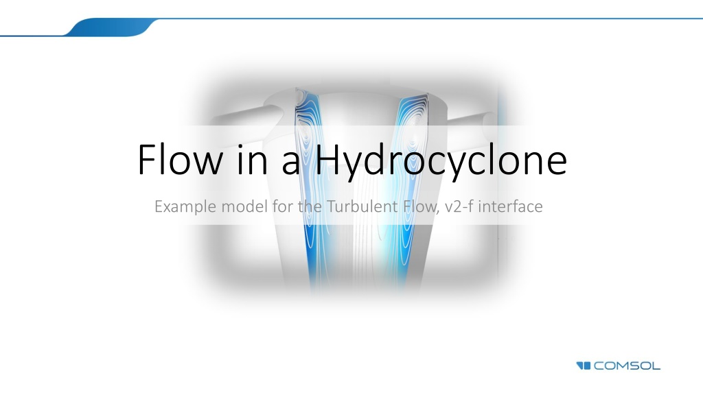
Flow in a Hydrocyclone Example model for the Turbulent Flow, v2-f interface
Model Overview Cyclones are used in a variety of applications ranging from the mining industry to vacuum cleaners. In the pulp and paper industry, hydrocyclones are used for several purposes including contaminant removal, pulp thickening and fiber fractionation. The flow in a hydrocyclone is characterized by a very strong swirl, which makes it difficult to simulate using isotropic turbulence models. In this tutorial model, the ?2 ? turbulence model is used to simulate the flow. It is imperative that the swirl flow is accurately captured in order to assess the separation efficiency for various particles. The resulting velocity field, and pressure drops between the inlets and the two outlets are both in qualitative and quantitative agreement with results in the literature.
Geometry Overflow The geometry was created in COMSOL by drawing the cross- section in a workplane, revolving it and forming a union with two cylindrical inlets. The two inlets, the overflow, underflow and vortex finder are shown in the figure. Inlet Inlet Vortex finder Underflow
Model Setup The flowing medium is water at 20 C. The initial values were chosen as zero velocity and zero pressure, and default values for the turbulence variables. No slip conditions with automatic wall treatment were applied on all walls. At the two inlets, the normal-flow velocity was set to 5[?/?]. Isotropic turbulence conditions with 5% turbulence intensity and a turbulence length scale equal to 0.07 times the inlet diameter were prescribed. A uniform pressure was applied at the overflow outlet and a constant outflow velocity corresponding to 5% of the total flow was applied at the underflow outlet(1). (1)More realistic outflow conditions can be simulated by attaching outlet chambers to the under- and overflow.
Mesh and Solver The mimimum element size on the domain had to be reduced to 0.4[??] and the minimum element size on the boundaries had to be reduced to 0.1[??] in order to comply with the geometry. The Algebraic Multigrid (AMG) was applied.
Results The streamlines describe a strong swirl-flow motion created in the annular inlet chamber. 95% of the flow (burgundy streamlines) reverses prior to reaching the underflow and instead exits through the overflow. Streamlines to the overflow (burgundy) and to the underflow (teal). Isosurface of vertical vorticity, displaying the vortex core.
Results The graph shows the azimuthal velocity component 10[??] below the vortex finder, clearly distinguishing a core with solid-body rotation from an outer, semi-free vortex. The pressure drop and the complex flow structure in the annular inlet chamber are shown in the plot to the right. Azimuthal velocity profile 10[cm] below the vortex finder Pressure drop and in-plane streamlines.
Summary The swirling flow in a hydrocyclone was simulated using the ?2 ? turbulence model. The shape of the azimuthal velocity profile, including a vortex core and an outer, semi-free vortex , was captured in the simulation. The flow field and pressure drops are in both qualitative and quantitative agreement with results from experiments and simulations on similar designs found in literature. Further studies could include adding particle tracing to study the separation efficiency, varying the flow rate, adding outlet chambers at the under- and overflow to examine the effect of outlet conditions, or changing the design.