Understanding Turbulence in Fluid Dynamics: A Comprehensive Exploration
Exploring the complexities of turbulence in fluid dynamics, from the Navier-Stokes equations to subgrid transport and turbulent diffusion. Insights into the transition from laminar to turbulent flow, subgrid scale importance, and treatment of small-scale eddies are discussed. The impact of turbulence on atmospheric phenomena and the parameterization of turbulent diffusion for small-scale eddies are also highlighted.

Download Presentation

Please find below an Image/Link to download the presentation.
The content on the website is provided AS IS for your information and personal use only. It may not be sold, licensed, or shared on other websites without obtaining consent from the author. Download presentation by click this link. If you encounter any issues during the download, it is possible that the publisher has removed the file from their server.
E N D
Presentation Transcript
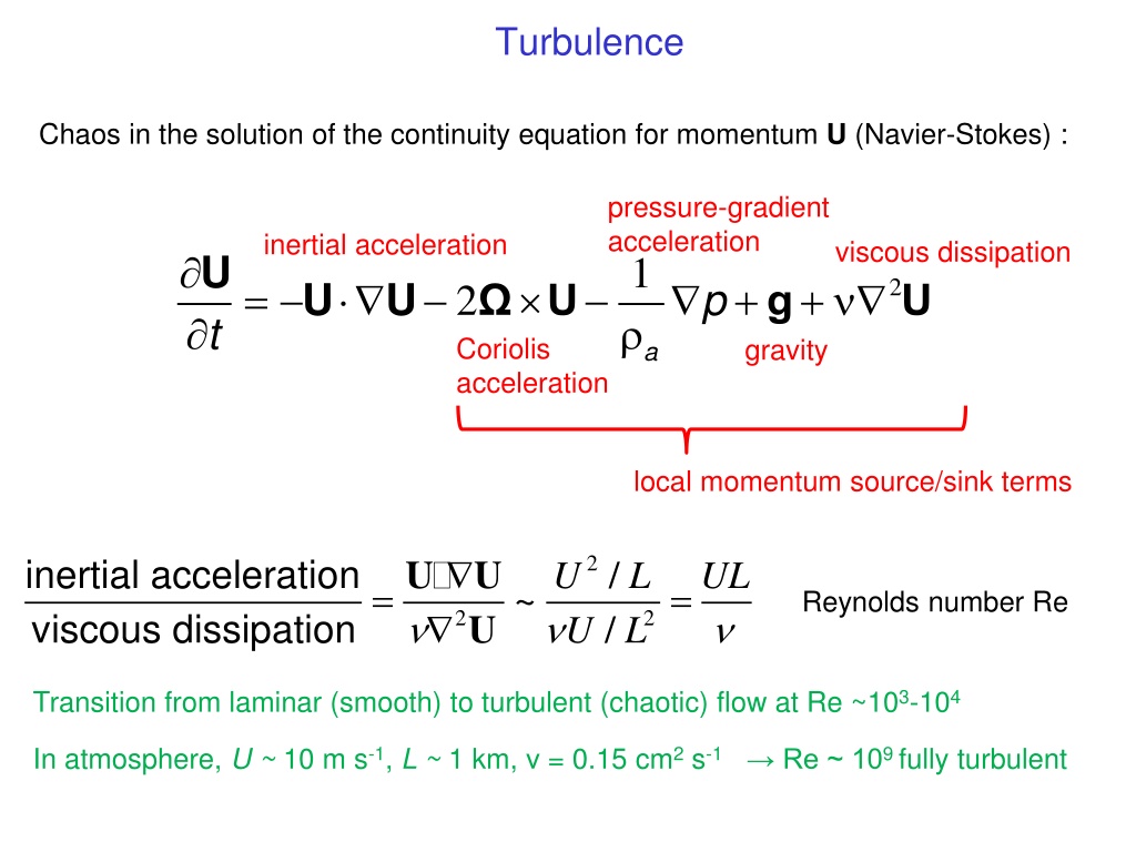
Turbulence Chaos in the solution of the continuity equation for momentum U (Navier-Stokes): pressure-gradient acceleration inertial acceleration viscous dissipation U t 1 = U + p + 2 U 2 Coriolis acceleration U g U gravity a local momentum source/sink terms 2 inertial acceleration viscous dissipation U U U / / U U L L UL = = ~ Reynolds number Re 2 2 Transition from laminar (smooth) to turbulent (chaotic) flow at Re ~103-104 In atmosphere, U ~ 10m s-1, L ~ 1 km, = 0.15 cm2 s-1 Re ~ 109 fully turbulent
Dealing with subgrid transport Atmospheric flow is turbulent down to mm scale where viscous dissipation (molecular diffusion) takes over Typical observations of surface wind (10 Hz) turbulent eddies Advection in models must cut off the subgrid scales: u = <u > + u instantaneous grid average fluctuating resolved unresolved (turbulent) deterministic stochastic Brasseur and Jacob, chap. 8.2
Importance of subgrid scales for mean transport Observations from Harvard Forest tower on a typical summer day tower (Bill Munger, Harvard) forest vertical wind w T CO2 (n) w = <w> + w n = <n> + n n Time-averaged vertical flux <F> = <nw> = <n><w> + <n w > ... . resolved turbulent (small) (large) .... w Turbulent flux is covariance between fluctuating components . Brasseur and Jacob, chap. 10.2.4
Turbulent diffusion parameterization for small-scale eddies = resolved turbulent implies Gaussian plumes for point sources C z F nw K n In 1-D (vertical) Kz is a turbulent diffusion coefficient, same for all species (similarity assumption) z z a California fire plumes, Oct 2004 Industrial plumes Generalized continuity equation in 3-D (Eulerian): K 0 0 0 x n t = + + n n C P L U K i = ( ) K K 0 0 with i a i i i y K 0 z Brasseur and Jacob, chap.8.4.1
Lagrangian treatment of small-scale eddies Treat turbulent component as Markov chain: = + 2 x u t K x x = + 2 y v t K y y position to+ t = w t + 2 z K z z where the random components have expected value of zero and standard deviation t ( ( x, y, z)T position to Brasseur and Jacob, chap. 4.11.2
Gaussian plume modeling of point source dispersion Point source with emission rate q Transport in cross-wind direction is parameterized as diffusive process: 2 2 C t C x C y C z = + + u K K for steady wind, inert plume y z 2 2 Turbulent diffusion coefficients Steady state solution with suitable boundary conditions: 2 2 q u y z K = + ( , , ) C x y z exp[ ( )] 4 ( 1/2 ) 4 K K x x K y z y z Brasseur and Jacob, chap. 4.12.1
Deep convection Subgrid in horizontal but organized in vertical Requires non-local parameterization of mass transport Convective cloud (0.1-100 km) z detrainment C-shaped profile for species with surface source Model vertical levels Large-scale subsidence downdraft updraft entrainment C Model grid scale Brasseur and Jacob, chap. 8.8
Question 1. Somewhat counterintuitively, representation of subgrid turbulent diffusion is more important in fine-resolution models than in coarse-resolution models. Why? That s because the turbulent diffusion parameterization (like molecular diffusion) is most efficient on small spatial scales. Consider a model grid cell: Rate constant for ventilation by advection: kA = u/ x Rate constant for ventilation by turbulent diffusion: kD =2K/( x)2 x advection turbulent diffusion k k u x K = = A Typical horizontal values u = 5 m s-1, K = 10 m2 s-1 2 Horizontal advection = turbulent diffusion for x = 4 km Typical vertical values w = 1 cm s-1, K = 10 m2 s-1 Turbulent diffusion dominates on any grid D But fine-resolution models can resolve large eddies (like deep convection) that are not amenable to turbulent diffusion parameterization. So coarse models are more in need of non-local turbulence parameterizations
Question 2. Satellites aim to quantify emissions from point sources by measuring concentrations in the plumes. Can these plume data be interpreted with a Gaussian plume model to infer the emissions? No, unless they are very large. Problem is that the observed plumes are instantaneous, i.e., a single realization of turbulence, whereas the Gaussian plume model assumes averaging over many realizations. Very large plumes experience these many realizations but small plumes don t. So we have to use different methods [Varon et al., AMT 2018] The same problem arises when predicting the downwind impacts of an instantaneous event (such as an explosion) Instantaneous methane plumes seen by GHGSat over Turkmenistan