Understanding One Factor Analysis of Variance (ANOVA)
One Factor Analysis of Variance (ANOVA) is a statistical method used to compare means of three or more groups. This method involves defining factors, measuring responses, examining assumptions, utilizing the F-distribution, and formulating hypothesis tests. ANOVA requires that populations are normally distributed, have equal standard deviations, and samples are randomly selected. The test statistic F is calculated based on between-sample and within-sample variances, and decisions are made by comparing it to critical values. The analysis of variance procedure involves determining if population means are equal through hypothesis testing, with implications for accepting or rejecting the null hypothesis based on significance levels.

Download Presentation

Please find below an Image/Link to download the presentation.
The content on the website is provided AS IS for your information and personal use only. It may not be sold, licensed, or shared on other websites without obtaining consent from the author. Download presentation by click this link. If you encounter any issues during the download, it is possible that the publisher has removed the file from their server.
E N D
Presentation Transcript
Inferential Statistics and Probability a Holistic Approach Chapter 12 One Factor Analysis of Variance (ANOVA) Creative Commons License This Course Material by Maurice Geraghty is licensed under a Creative Commons Attribution-ShareAlike 4.0 International License. Conditions for use are shown here: https://creativecommons.org/licenses/by-sa/4.0/ 1
ANOVA Definitions Factor categorical variable that defines the populations. Response variable that is being measured. Levels the number of choices for the factor, represented by k Replicates the sample size for each level, n1, n2, , nk. If n1 = n2 = = nk , then the design is balanced. Ho: There is no difference in the mean <response in context> due to the <factor in context>. Ha: There is a difference in the mean <response in context> due to the <factor in context>. 2
11-8 Underlying Assumptions for ANOVA The F distribution is also used for testing the equality of more than two means using a technique called analysis of variance (ANOVA). ANOVA requires the following conditions: The populations being sampled are normally distributed. The populations have equal standard deviations. The samples are randomly selected and are independent. 3
11-3 Characteristics of F- Distribution There is a family of F Distributions. Each member of the family is determined by two parameters: the numerator degrees of freedom and the denominator degrees of freedom. F cannot be negative, and it is a continuous distribution. The F distribution is positively skewed. Its values range from 0 to . As F the curve approaches the X-axis. 4
11-9 Analysis of Variance Procedure The Null Hypothesis: the population means are the same. The Alternative Hypothesis: at least one of the means is different. The Test Statistic: F=(between sample variance)/(within sample variance). Decision rule: For a given significance level , reject the null hypothesis if F (computed) is greater than F (table) with numerator and denominator degrees of freedom. 5
ANOVA Null Hypothesis Ho is false -not all means the same Ho is true -all means the same 6
11-10 ANOVA NOTES If there are k populations being sampled (levels), then the dffactor = k-1 If the sample size is n, then dferror= n-k The test statistic is computed by:F=[(SSF)/(k-1)]/[(SSE)/(n-k)]. SSF represents the factor (between) sum of squares. SSE represents the error (within) sum of squares. Let TC represent the column totals, nc represent the number of observations in each column, and X represent the sum of all the observations. These calculations are tedious, so technology is used to generate the ANOVA table. 7
11-11 Formulas for ANOVA ( ) 2 ( ) X = 2 SS X Total n ( ) 2 2 T X = c SS Factor n n c = SS SS SS Error Total Factor 8
ANOVA Table Source SS df MS F Factor SSFactor k-1 SSF/dfF MSF/MSE Error SSError n-k SSE/dfE Total SSTotal n-1 9
11-12 EXAMPLE Party Pizza specializes in meals for students. Hsieh Li, President, recently developed a new tofu pizza. Before making it a part of the regular menu she decides to test it in several of her restaurants. She would like to know if there is a difference in the mean number of tofu pizzas sold per day at the Cupertino, San Jose, and Santa Clara pizzerias for sample of five days. At the .05 significance level can Hsieh Li conclude that there is a difference in the mean number of tofu pizzas sold per day at the three pizzerias? 10
Example Cupertino 13 12 14 12 San Jose 10 12 13 11 Santa Clara 18 16 17 17 17 85 5 17 1447 Total T n 51 4 46 4 11.5 534 182 13 14 2634 Means ^2 12.75 653 11
Example continued 2 182 = = 2634 86 SS Total 13 2 182 = = 2624 25 . 76 25 . SS Factor 13 = = SS 8 6 . 6 7 25 . 9 75 Error 12
Example 4 continued ANOVA TABLE Source SS df MS F Factor 76.25 2 38.125 39.10 Error 9.75 10 0.975 Total 86.00 12 13
11-14 EXAMPLE 4 continued Design: Ho: 1= 2= 3 Ha: Not all the means are the same =.05 Model: One Factor ANOVA H0 is rejected if F>4.10 Data: Test statistic: F=[76.25/2]/[9.75/10]=39.1026 H0 is rejected. Conclusion: There is a difference in the mean number of pizzas sold at each pizzeria. 14
Post Hoc Comparison Test Used for pairwise comparison Designed so the overall signficance level is 5%. Use technology. Refer to Tukey Test Material in the textbook. 16
Example Oranges & Orchards Valencia oranges were tested for juiciness at 4 different orchards. Eight oranges were sampled from each orchard, and the total ml of juice per 20 gms of orange was calculated. Test for a difference in juiciness due to orchards using alpha = .05 Perform all the pairwise comparisons using Tukey's Test and an overall risk level of 5%. 19
Example - Defintions Factor: Orchard (A, B, C or D) Response: Juiciness of orange Levels: k = 4 Replicate: nA = nB = nC = nD = 8 Design: Balanced Sample size: n = 8 + 8 + 8 + 8 = 32 20