Understanding Analysis of Variance (ANOVA) for Testing Multiple Group Differences

Testing for differences among three or more groups can be effectively done using Analysis of Variance (ANOVA). By focusing on variance between means, ANOVA allows for comparison of multiple groups while avoiding issues of dependence and multiple comparisons. Sir Ronald Fisher's ANOVA method provides a statistical approach to test hypotheses regarding mean differences across multiple groups.

• ANOVA
• Analysis of Variance
• Group Differences
• Hypothesis Testing
• Sir Ronald Fisher

tycho Follow

Uploaded on Jul 19, 2024 | 0 Views

Download Presentation

Please find below an Image/Link to download the presentation.

The content on the website is provided AS IS for your information and personal use only. It may not be sold, licensed, or shared on other websites without obtaining consent from the author. Download presentation by click this link. If you encounter any issues during the download, it is possible that the publisher has removed the file from their server.

Presentation Transcript

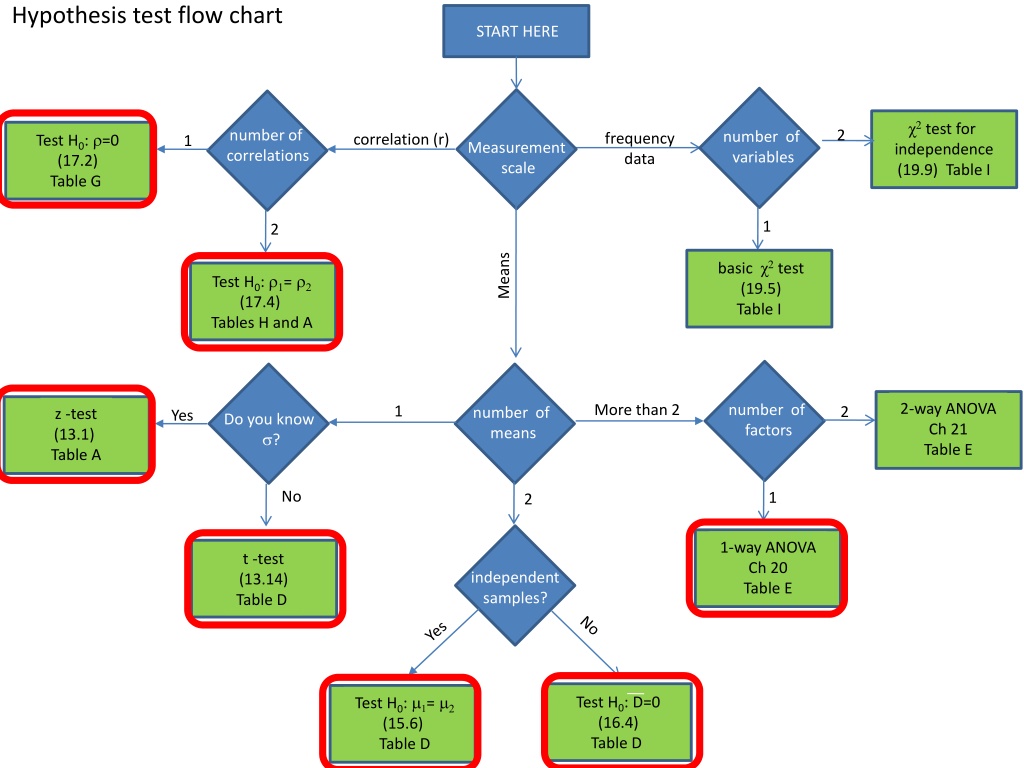
1. Hypothesis test flow chart START HERE 2 test for independence (19.9) Table I 2 number of correlations Test H0: =0 (17.2) Table G number of variables frequency data correlation (r) 1 Measurement scale 1 2 Means basic 2 test (19.5) Table I Test H0: = (17.4) Tables H and A 2-way ANOVA Ch 21 Table E More than 2 number of factors 1 2 number of means z -test (13.1) Table A Yes Do you know ? No 1 2 1-way ANOVA Ch 20 Table E t -test (13.14) Table D independent samples? Test H0: = (15.6) Table D Test H0: D=0 (16.4) Table D

2. Chapter 18: Testing for difference among three or more groups: One way Analysis of Variance (ANOVA) A B C Suppose you wanted to compare the results of three tests (A, B and C) to see if there was any differences difficulty. To test this, you randomly sample these ten scores from each of the three populations of test scores. 84 85 62 78 62 79 93 62 83 76 74 79 92 71 80 68 81 74 How would you test to see if there was any difference across the mean scores for these three tests? 79 69 84 76 87 67 81 68 67 The first thing is obvious calculate the mean for each of the three samples of 10 scores. 87 61 75 Means But then what? You could run three two-sample t-tests on each of the pairs (A vs. B, A vs. C and B vs. C). 81 72 75

3. A B C You could run an two-sample t-test on each of the pairs (A vs. B, A vs. C and B vs. C). 84 85 62 78 62 79 93 62 83 76 74 79 There are two problems with this: 92 71 80 68 81 74 1) The three tests wouldn t be truly independent of each other, since they contain common values, and 79 69 84 76 87 67 81 68 67 2) We run into the problem of making multiple comparisons: If we use an value of .05, the probability of obtaining at least one significant comparison by chance is 1-(1-.05)3, or about .14 87 61 75 Means 81 72 75 So how do we test the null hypothesis: H0: A = B = C ?

4. So how do we test the null hypothesis: H0: A = B = C ? In the 1920 s Sir Ronald Fisher developed a method called Analysis of Variance or ANOVA to test hypotheses like this. A B C 84 85 62 The trick is to look at the amount of variability between the means. 78 62 79 93 62 83 76 74 79 So far in this class, we ve usually talked about variability in terms of standard deviations. ANOVA s focus on variances instead, which (of course) is the square of the standard deviation. The intuition is the same. 92 71 80 68 81 74 79 69 84 76 87 67 81 68 67 The variance of these three mean scores (81, 72 and 75) is 22.5 87 61 75 Means Intuitively, you can see that if the variance of the means scores is large , then we should reject H0. 81 72 75 But what do we compare this number 22.5 to?

5. So how do we test the null hypothesis: H0: A = B = C ? The variance of these three mean scores (81, 72 and 75) is 22.5 How large is 22.5? A B C 84 85 62 Suppose we knew the standard deviation of the population of scores ( ). 78 62 79 93 62 83 76 74 79 If the null hypothesis is true, then all scores across all three columns are drawn from a population with standard deviation . 92 71 80 68 81 74 79 69 84 76 87 67 It follows that the mean of n scores should be drawn from a population with standard deviation: 81 68 67 87 61 75 Means = n 2 2 = Xs sX With a little algebra: n 81 72 75 This means multiplying the variance of the means by n gives us an estimate of the variance of the population.

6. The variance of these three mean scores (81, 72 and 75) is 22.5 Multiplying the variance of the means by n gives us an estimate of the variance of the population. = = 2 10 ( )( 22 ) 5 . 225 A B C n Xs For our example, 84 85 62 78 62 79 We typically don t know what is. But like we do for t-tests, we can use the variance within our samples to estimate it. The variance of the 10 numbers in each column (61, 94, and 55) should each provide an estimate of . 93 62 83 76 74 79 92 71 80 68 81 74 79 69 84 We can combine these three estimates of by taking their average, which is 70. 76 87 67 81 68 67 87 61 75 Means n x Variance of means 81 72 75 225 Variances Mean of variances 61 94 55 70

7. If H0: A = B = C is true, we now have two separate estimates of the variance of the population ( ). One is n times the variance of the means of each column. The other is the mean of the variances of each column. A B C 84 85 62 If H0 is true, then these two numbers should be, on average, the same, since they re both estimates of the same thing ( ). 78 62 79 93 62 83 76 74 79 For our example, these two numbers (225 and 70) seem quite different. 92 71 80 68 81 74 Remember our intuition that a large variance of the means should be evidence against H0. Now we have something to compare it to. 225 seems large compared to 70. 79 69 84 76 87 67 81 68 67 87 61 75 Means n x Variance of means 81 72 75 225 Variances Mean of variances 61 94 55 70

8. When conducting an ANOVA, we compute the ratio of these two estimates of . This ratio is called the F statistic . For our example, 225/70 = 3.23. If H0 is true, then the value of F should be around 1. If H0 is not true, then F should be significantly greater than 1. A B C 84 85 62 We determine how large F should be for rejecting H0 by looking up Fcrit in Table E. F distributions depend on two separate degrees of freedom one for the numerator and one for the denominator. 78 62 79 93 62 83 76 74 79 92 71 80 df for the numerator is k-1, where k is the number of columns or treatments . For our example, df is 3-1 =2. 68 81 74 79 69 84 76 87 67 df for the denominator is N-k, where N is the total number of scores. In our case, df is 30-3 = 27. 81 68 67 87 61 75 Fcrit for = .05 and df s of 2 and 27 is 3.35. Means n x Variance of means 81 72 75 225 Ratio (F) 3.23 Variances Mean of variances Since Fobs = 3.23 is less than Fcrit, we fail to reject H0. We cannot conclude that the exam scores come from populations with different means. 61 94 55 70

9. Fcrit for = .05 and dfs of 2 and 27 is 3.35. Since Fobs = 3.23 is less than Fcrit, we fail to reject H0. We cannot conclude that the exam scores come from populations with different means. Instead of finding Fcrit in Table E, we could have calculated the p-value using our F- calculator. Reporting p-values is standard. Our p-value for F=3.23 with 2 and 27 degrees of freedom is p=.0552 Since our p-value is greater then .05, we fail to reject H0

10. Example: Consider the following n=12 samples drawn from k=5 groups. Use an ANOVA to test the hypothesis that the means of the populations that these 5 groups were drawn from are different. A B C D E Answer: The 5 means and variances are calculated below, along with n x variance of means, and the mean of variances. 68 84 97 79 82 61 67 97 72 90 84 67 76 69 78 78 75 107 76 65 Our resulting F statistic is 15.32. 93 85 111 74 65 76 62 104 66 79 92 62 87 78 72 Our two dfs are k-1=4 (numerator) and 60-5 = 55(denominator). Table E shows that Fcrit for 4 and 55 is 2.54. 68 74 104 83 81 79 71 108 91 86 76 81 104 75 64 81 69 105 70 51 Fobs > Fcrit so we reject H0. 87 87 99 78 91 Means n x Variance of means 78 74 100 76 75 1429 Ratio (F) 15.32 Variances Mean of variances 96 78 97 46 149 93

11. What does the probability distribution F(dfbet,dfw) look like? F(2,5) F(2,10) F(2,50) F(2,100) 0 1 2 3 4 5 0 1 2 3 4 5 0 1 2 3 4 5 0 1 2 3 4 5 F(10,5) F(10,10) F(10,50) F(10,100) 0 1 2 3 4 5 0 1 2 3 4 5 0 1 2 3 4 5 0 1 2 3 4 5 F(50,5) F(50,10) F(50,50) F(50,100) 0 1 2 3 4 5 0 1 2 3 4 5 0 1 2 3 4 5 0 1 2 3 4 5

12. For a typical ANOVA, the number of samples in each group may be different, but the intuition is the same - compute F which is the ratio of the variance of the means over the mean of the variances. Formally, the variance is divided up the following way: Given a table of k groups, each containing ni scores (i= 1,2, , k), we can represent the deviation of a given score, X from the mean of all scores, called the grand mean as: = + ( ) ( ) X X X X X X Deviation of X from the grand mean Deviation of X from the mean of the group Deviation of the mean of the group from the grand mean

13. The total sums of squares can be partitioned into two numbers: all all scores scores k = i = + 2 2 2 ( ) ( ) ( ) X X X X n X X i 1 Between-groups sum of squares: SSbet Total sum of squares: SStotal Within-groups sum of squares: SSw SSbet is a measure of the variability between groups. It is used as the numerator in our F-tests The variance between groups, called mean squared error , or MSbet, is calculated by dividing SSbet by its degrees of freedom dfbet = k-1 MSbet=SSbet/dfbet and is another estimate of 2 if H0 is true. This is essentially n times the variance of the means. . If H0 is not true, then s2bet is an estimate of 2 plus any treatment effect that would add to a difference between the means.

14. The total sums of squares can be partitioned into two numbers: all all scores scores k = i = + 2 2 2 ( ) ( ) ( ) X X X X n X X i 1 Between-groups sum of squares: SSbet Total sum of squares: SStotal Within-groups sum of squares: SSw SSwis a measure of the variability within each group. It is used as the denominator in all F-tests. The variance within each group, MSw is calculated by dividing SSw by its degrees of freedom dfw = ntotal k MSw=SSw/dfw This is an estimate of 2 This is essentially the mean of the variances within each group. (It is exactly the mean of variances if our sample sizes are all the same.)

15. The F ratio is calculated by dividing up the sums of squares and df into between and within SStotal = SSw + SSbet Variances are then calculated by dividing SS by df all MSbet=SSbet/dfbet scores SStotal 2) ( X X MSw=SSw/dfw SSw SSbet F is the ratio of variances between and within all k = i scores 2) ( n X X 2) ( X X F=????? ??? i 1 dftotal = dfw + dfbet dftotal =ntotal-1 dfw =ntotal-k dfbet =k-1

16. Finally, the F ratio is the ratio of MSbet and MSw F=????? ??? We can write all these calculated values in a summary table like this: Source SS df MS F ????? ??? k = i 2) ( n X X MSbet=SSbet/dfbet Between k-1 i 1 all scores MSw=SSw/dfw Within ntotal-k 2) ( X X all scores Total ntotal-1 2) ( X X (k is the number of groups)

17. A B C D E Calculating SStotal 68 84 97 79 82 61 67 97 72 90 4839= 84 67 76 69 78 = 80 7 . X grand mean: 60 78 75 107 76 65 93 85 111 74 65 k = i 76 62 104 66 79 = + + 2 2 2 ( ) ( 68 80 ) 7 . ( 61 80 ) 7 . ... SS X X total 92 62 87 78 72 = 1 68 74 104 83 81 + = 2 91 ( 80 ) 7 . 10847 79 71 108 91 86 76 81 104 75 64 81 69 105 70 51 87 87 99 78 91 Means n x Variance of means 78 74 100 76 75 1429 Ratio (F) 15.32 Variances Mean of variances 96 78 97 46 149 93 Source SS df MS F Between Within Total 10847 59

18. A B C D E Calculating SSbet and MSbet 68 84 97 79 82 61 67 97 72 90 4839= = 80 7 . X 84 67 76 69 78 60 78 75 107 76 65 93 85 111 74 65 k = i = + + 2 2 2 ( ) 12 ( )( 78 80 ) 7 . 12 ( )( 74 80 ) 7 . ... SS n X X 76 62 104 66 79 bet i 92 62 87 78 72 = 1 68 74 104 83 81 + = 2 12 ( )( 75 80 ) 7 . 5717 79 71 108 91 86 76 81 104 75 64 ?????=????? ?????=5717 4=1429 81 69 105 70 51 87 87 99 78 91 Means n x Variance of means 78 74 100 76 75 1429 Ratio (F) 15.32 Variances Mean of variances 96 78 97 46 149 93 Source SS df MS F Between 5717 5-1=4 1429 Within Total 10847 59

19. A B C D E Calculating SSw and MSw 68 84 97 79 82 61 67 97 72 90 84 67 76 69 78 k = i = + + 2 2 2 ( ) 68 ( 78 ) ( 61 78 ) ... SS X X 78 75 107 76 65 w 93 85 111 74 65 = 1 76 62 104 66 79 + + + + = 2 2 2 84 ( 74 ) ( 67 74 ) ... 91 ( 75 ) 5130 92 62 87 78 72 68 74 104 83 81 ???=??? ???=5130 79 71 108 91 86 55=93 76 81 104 75 64 81 69 105 70 51 87 87 99 78 91 Means n x Variance of means 78 74 100 76 75 1429 Ratio (F) 15.32 Variances Mean of variances 96 78 97 46 149 93 Source SS df MS F Between 5717 5-1=4 1429 Within 5130 12x5-5=55 93 Total 10847 59

20. A B C D E Calculating F 68 84 97 79 82 61 67 97 72 90 84 67 76 69 78 F=????? ???=1429 93= 15.32 78 75 107 76 65 93 85 111 74 65 76 62 104 66 79 92 62 87 78 72 Fcrit with dfs of 4 and 55 and = .05 is 2.54 68 74 104 83 81 79 71 108 91 86 Our decision is to reject H0 since 15.32 > 2.54 76 81 104 75 64 81 69 105 70 51 87 87 99 78 91 Means n x Variance of means 78 74 100 76 75 1429 Ratio (F) 15.32 Variances Mean of variances 96 78 97 46 149 93 Source SS df MS F Between 5717 5-1=4 1429 15.32 Within 5130 12x5-5=55 93 Total 10847 59