Understanding Variance and Covariance in Probabilistic System Analysis
Variance and covariance play crucial roles in probabilistic system analysis. Variance measures the variability in a probability distribution, while covariance describes the relationship between two random variables. This lecture by Dr. Erwin Sitompul at President University delves into these concepts with examples and explanations, highlighting their significance in analyzing uncertainties and data distributions.

Download Presentation

Please find below an Image/Link to download the presentation.
The content on the website is provided AS IS for your information and personal use only. It may not be sold, licensed, or shared on other websites without obtaining consent from the author. Download presentation by click this link. If you encounter any issues during the download, it is possible that the publisher has removed the file from their server.
E N D
Presentation Transcript
Probabilistic System Analysis Lecture 5 Dr.-Ing. Erwin Sitompul President University http://zitompul.wordpress.com 2 0 2 1 President University Erwin Sitompul PSA 5/1
Chapter 4.2 Variance and Covariance Variance The mean or expected value of a random variable X is important because it describes the center of the probability distribution. However, the mean does not give adequate description of the shape and variability in the distribution. Distribution with equal means but different dispersions (variability) The most important measure of variability of a random variable X is obtained by letting g(X) = (X )2. This variability measure is referred to as the variance of the random variable Xor the variance of the probability distribution of X. It is denoted by Var(X) or the symbol , or simply by . 2 X 2 President University Erwin Sitompul PSA 5/2
Chapter 4.2 Variance and Covariance Variance Let X be a random variable with probability distribution f(x) and mean . The variance of X is if X is discrete, and = = 2 2 2 [( ) ] ( ) ( ) f x E X x x = = 2 2 2 [( ) ] ( ) ( ) f x dx E X x if X is continuous. The positive square root of the variance, , is called the standard deviation of X. President University Erwin Sitompul PSA 5/3
Chapter 4.2 Variance and Covariance Variance Company A Let the random variable X represent the number of cars that are used for official business purposes on any given workday. The probability distribution for company A and company B are Company B Show that the variance of the probability distribution for company B is greater than that of company A. = = + + = ( ) E X (1)(0.3) (2)(0.4) (3)(0.3) 2 3 = = = (1 2) (0.3) + + 2 2 2 2 2 ( 2) ( ) f x x 0.6 (2 2) (0.4) (3 2) (0.3) = 1 x = = + + + + = ( ) E X 3 (0)(0.2) (1)(0.1) (2)(0.3) (3)(0.3) (4)(0.1) 2 = = + + = 2 2 2 2 2 ( 2) ( ) f x x (0 2) (0.3) (1 2) (0.3) (2 2) (0.4) (3 2) (0.3) (4 2) (0.3) + + 1.6 2 2 = 1 x Clearly, the variance of the number of cars that are used for official business purposes is greater for company B than for company A. President University Erwin Sitompul PSA 5/4
Chapter 4.2 Variance and Covariance Variance The variance of a random variable X is also given by ( ) E X = 2 2 2 Let the random variable X represent the number of defective parts for a machine when 3 parts are sampled from a production line and tested. The following is the probability distribution of X Calculate the variance 2. = + + + = (0)(0.51) (1)(0.38) (2)(0.10) (3)(0.01) 0.61 3 = = (0) (0.51) (1) (0.38) (2) (0.10) (3) (0.01) + + + = 2 2 2 2 2 2 ( ) ( ) 0.87 E X x f x = 0 x = = = 2 2 2 2 0.4979 ( ) 0.87 (0.61) E X President University Erwin Sitompul PSA 5/5
Chapter 4.2 Variance and Covariance Variance The weekly demand for a drinking-water product, in thousands liters, from a local chain of efficiency stores, is a continuous random variable X having the probability density 0, elsewhere 2( 1), 1 2 x x = ( ) f x Find the mean and variance of X. 2 2 2 3x 5 3 = 3 2 = = x 2( 1) x x dx 1 1 2 2 2 4 2 3 17 6 = 4 3 = = 2 2 x x ( ) 2( 1) E X x x dx 1 1 2 17 6 5 3 1 = = = 2 2 2 ( ) E X 18 President University Erwin Sitompul PSA 5/6
Chapter 4.2 Variance and Covariance Variance Let X be a random variable with probability distribution f(x). The variance of the random variable g(X) is if X is discrete, and = = 2 g X 2 2 {[ ( ) E g X ] } [ ( ) g X ] ( ) f x ( ) ( ) ( ) g X g X x = = 2 g X 2 2 {[ ( ) E g X ] } [ ( ) g X ] ( ) f x dx ( ) ( ) ( ) g X g X if X is continuous. President University Erwin Sitompul PSA 5/7
Chapter 4.2 Variance and Covariance Variance Calculate the variance of g(X) = 2X+3, where X is a random variable with probability distribution given as 3 1 4 1 8 1 2 1 8 + + + = = = + = (3) (5) (7) (9) 6 (2 3) ( ) f x x + ( ) 2 3 g X X = 0 x = = + 3) 6] } 2 g X 2 2 {[ ( ) E g X ] } {[(2 E X ( ) ( ) g X 3 = + = + 2 2 [4 12 9] (4 12 9) ( ) f x E X X x x = 0 x 1 4 1 8 1 2 1 8 = + + + = (9) (1) (1) (9) 4 President University Erwin Sitompul PSA 5/8
Chapter 4.2 Variance and Covariance Variance Let X be a random variable with density function 2 , 1 ( ) 3 0, elsewhere x 2 x = f x Find the variance of the random variable g(X)=4X+3 if it is known that the expected value of g(X) = 8. += + 3) 8] } = + 2 4 2 2 {[(4 E [16 E 40 25] X X X 3 X 2 2 2 x = + 2 = + 2 (16 40 25) x x dx (16 40 25) ( ) f x dx x x 3 1 1 2 2 1 16 3 51 5 40 4 25 3 1 3 1 136 3 15 = + = + 5 4 3 4 3 2 x x x 16 40 25 x x x dx 5 1 1 323 15 459 45 = = = President University Erwin Sitompul PSA 5/9
Chapter 4.2 Variance and Covariance Covariance Let X and Y be a random variables with probability distribution f(x,y). The covariance of the random variables X and Y is if X and Y arediscrete, and = = [( )( )] ( )( ) ( , ) f x y E X Y x y XY X Y X Y x y = = [( )( )] ( )( ) ( , ) f x y dxdy E X Y x y XY X Y X Y if X and Y are continuous. XY >0, Positive covariance XY <0 Negative covariance President University Erwin Sitompul PSA 5/10
Chapter 4.2 Variance and Covariance Covariance The covariance of two random variables X and Y with means X and Y, respectively, is given by ( ) XY X Y E XY = President University Erwin Sitompul PSA 5/11
Chapter 4.2 Variance and Covariance Covariance Referring back again to the ballpoint pens example, find the covariance of X and Y. 2 5 15 28 3 28 3 4 2 2 = = = + + = = ( ) (0) (1) (2) xg x ( ) E X ( , ) xf x y X 14 = 0 x = = 0 0 x y 2 2 2 15 28 3 7 1 28 1 2 = = = + + = = (0) (1) (2) ( ) ( , ) yf x y ( ) E Y yh y Y = = = 0 0 0 x y y 3 3 4 1 2 9 = = = ( ) E XY XY X Y 14 56 See again Lecture 4 President University Erwin Sitompul PSA 5/12
Chapter 4.2 Variance and Covariance Covariance The fraction X of male runners and the fraction Y of female runners who compete in marathon races is described by the joint density function 0, elsewhere Find the covariance of X and Y 8 , 0 1 xy y x = ( , ) f x y = = ( ) g x ( , ) f x y dy ( ) h y ( , ) f x y dx and 1 1 4 9 3 4 0, , 0 1 x x = = = ( ) (8 ) E XY xy xy dxdy ( ) g x elsewhere 0 y 2 4 (1 0, ), 0 1 y y y = ( ) h y = ( ) E XY elsewhere XY X Y 4 9 4 5 8 4 1 4 5 = = = = = 4 ( ) E X 4 x dx 15 225 X 0 1 8 = = 2 2 = ( ) 4 (1 ) E Y y y dy Y 15 0 President University Erwin Sitompul PSA 5/13
Chapter 4.2 Variance and Covariance Covariance Although the covariance between two random variables does provide information regarding the nature of the relationship, the magnitude of XYdoes not indicate anything regarding the strength of the relationship, since XY is not scale free. This means, that its magnitude will depend on the units measured for both X and Y. There is a scale-free version of the covariance called the correlation coefficient, that is used widely in statistics. Let X and Y be random variables with covariance XY and standard deviation X and Y, respectively. The correlation coefficientX and Y is = XY XY X Y President University Erwin Sitompul PSA 5/14
Chapter 4.3 Means and Variances of Linear Combinations of Random Variables Means of Linear Combinations of X If a and b are constant, then ( ) ( ) E aX b aE X b + = + Applying theorem to the discrete random variable g(X) = 2X 1, rework the carwash example. = (2 1) 2 ( ) 1 E X E X 9 = = ( ) E X ( ) xf x X = 4 x 1 1 1 4 1 4 1 6 1 6 41 6 = + + + + + = (4) (5) (6) (7) (8) (9) 12 12 41 6 = = = 2 1 $12.67 2 1 2 1 X X President University Erwin Sitompul PSA 5/15
Chapter 4.3 Means and Variances of Linear Combinations of Random Variables Means of Linear Combinations of X Let X be a random variable with density function 2 , 1 2 ( ) 3 0, elsewhere x x = f x Find the expected value of g(X)=4X+3 by using the theorem presented recently. + = + (4 3) 4 ( ) 3 E X E X 2 2 3 2 5 4 xdx x = = = ( ) E X x dx 3 3 1 1 5 4 + = + = (4 3) 4 3 8 E X President University Erwin Sitompul PSA 5/16
Chapter 4.3 Means and Variances of Linear Combinations of Random Variables Means of Linear Combinations of X The expected value of the sum or difference of two or more functions of a random variable X is the sum or difference of the expected values of the functions. That is [ ( ) ( )] [ ( )] [ ( )] E g X h X E g X E h X = Let X be a random variable with probability distribution as given next. Find the expected value of Y=(X 1)2. = + = ) 2 ( ) E X + 2 2 2 [( 1) ] [ 2 1] ( (1) E X E X X E X E 1 3 1 2 1 6 = + + + = ( ) E X (0) (1) (2)(0) (3) 1 1 3 1 2 1 6 = + + + = 2 2 2 2 ( ) (0) (1) (2) (0) (3) 2 E X E X 2 (2)(1) 1 = + = 2 [( 1) ] 1 President University Erwin Sitompul PSA 5/17
Chapter 4.3 Means and Variances of Linear Combinations of Random Variables Means of Linear Combinations of X The weekly demand for a certain drink, in thousands of liters, at a chain of convenience stores is a continuous random variable g(X) = X2+X 2, where X has the density function 0, elsewhere Find the expected value for the weekly demand of the drink. 2( 1), 1 2 x x = ( ) f x + = + 2 2 ( 2) ( ) ( ) E X (2) E X X E X E 2 2 5 3 = = = 2 2 ( ) x x dx ( ) E X 2 ( x x 1) dx 1 1 2 2 17 3 = = = 2 2 3 2 ( ) 2 ( 1) 2 ( ) E X x x dx x x dx 1 1 17 6 5 3 5 2 + = 2 + = ( 2) E X X 2 President University Erwin Sitompul PSA 5/18
Chapter 4.3 Means and Variances of Linear Combinations of Random Variables Means of Linear Combinations of X and Y The expected value of the sum or difference of two or more functions of a random variables X and Y is the sum or difference of the expected values of the functions. That is ( , ) ( , ) ( , ) E g X Y h X Y E g X Y = ( , ) E h X Y Let X and Y be two independent random variables. Then ( ) ( ) ( ) E XY E X E Y = President University Erwin Sitompul PSA 5/19
Chapter 4.3 Means and Variances of Linear Combinations of Random Variables Means of Linear Combinations of X and Y In producing gallium-arsenide microchips, it is known that the ratio between gallium and arsenide is independent of producing a high percentage of workable wafers, which are the main components of microchips. Let X denote the ratio of gallium to arsenide and Y denote the percentage of workable microwafers retrieved during a 1-hour period. X and Y are independent random variables with the joint density being known as + = Illustrate that E(XY) = E(X)E(Y). 2 (1 3 ), 0 x y 2, 0 1 x y ( , ) f x y 4 0, elsewhere 1 2 1 2 + 2 2 (1 3 4 2 (1 3 y ) x y y = = ( ) ( , ) E XY xyf x y dxdy dxdy 0 0 1 0 0 = 2 x 1 + 2 + ) 5 6 y 3 2 (1 3 12 ) x y y = = = dy dy 3 0 0 = 0 x President University Erwin Sitompul PSA 5/20
Chapter 4.3 Means and Variances of Linear Combinations of Random Variables Means of Linear Combinations of X and Y 1 2 1 2 + 2 2 (1 3 4 ) x y = = ( ) E X ( , ) xf x y dxdy dxdy 0 0 0 0 = 2 x 1 1 + + 3 2 2 (1 3 12 ) x y 2(1 3 ) 4 3 y = = = dy dy 3 0 0 = 0 x 1 2 1 2 + 2 (1 3 4 ) xy y = = ( ) ( , ) yf x y dxdy E Y dxdy 0 0 0 0 = 2 x 1 1 + (1 3 + 2 2 2 (1 3 8 ) ) 5 8 x y y y y = = = dy dy 2 0 0 = 0 x Hence, it is proven that 5 6 4 3 5 8 = = = ( ) ( ) E X ( ) E XY E Y President University Erwin Sitompul PSA 5/21
Chapter 4.3 Means and Variances of Linear Combinations of Random Variables Means of Linear Combinations of X and Y If a and b are constant, then a a = += 2 aX b 2 2 X 2 2 If X and Y are random variables with joint probability distribution f(x,y), then 2 2 2 2 2 2 aX bY X Y XY a b ab + = + + President University Erwin Sitompul PSA 5/22
Chapter 4.3 Means and Variances of Linear Combinations of Random Variables Means of Linear Combinations of X and Y = = 2 X 2 Y 2 4 If X and Y are random variables with variances , , and covariance XY = 2, find the variance of the random variable Z = 3X 4Y+8. = + = = = = (9)(2) (16)(4) (24)( 2) + 130 2 X 2 Y 2 Z 2 3 2 3 9 16 24 + 4 8 4 XY X Y X Y Let X and Y denote the amount of two different types of impurities in a batch of a certain chemical product. Suppose that X and Y are independent random variables with variances and . Find the variance of the random variable Z = 3X 2Y + 5. = = 2 X 2 Y 2 3 = = = + = (9)(2) (4)(3) + 2 Z 2 3 2 3 2 X 2 Y 9 4 + 2 5 2 X Y X Y = 30 President University Erwin Sitompul PSA 5/23
Chapter 4.4 Chebyshev s Theorem Chebyshev s Theorem As we already discussed, the variance of a random variable tells us something about the variability of the observation about the mean. If a variable has a small variance or standard deviation, we would expect most of the values to be grouped around the mean. The probability that a random variable assumes a value within a certain interval about the mean is greater in this case. If we think of probability in terms of area, we would expect a continuous distribution with a small standard deviation to have most of its area close to . Small , less variability Large , more variability Variability of continuous observations about the mean President University Erwin Sitompul PSA 5/24
Chapter 4.4 Chebyshev s Theorem Chebyshev s Theorem We can argue the same way for a discrete distribution. The spread out of an area in the probability histogram indicates a more variable distribution of measurements or outcomes. Small , less variability Large , more variability Variability of discrete observations about the mean President University Erwin Sitompul PSA 5/25
Chapter 4.4 Chebyshev s Theorem Chebyshev s Theorem A Russian mathematician P. L. Chebyshev discovered that the fraction of the area between any two values symmetric about the mean is related to the standard deviation. |Chebyshev s Theorem| The probability that any random variable X will assume a value within k standard deviations of the mean is at least 1 1/k2. That is 1 ( ) 1 P k X k k + 2 Chebyshev s Theorem holds for any distribution of observations and, for this reason, the results are usually weak. The value given by the theorem is a lower bound only. Exact probabilities can only be determined when the probability distribution is known. The use of Chebyshev s Theorem is relegated to situations where the form of the distribution is unknown. President University Erwin Sitompul PSA 5/26
Chapter 4.4 Chebyshev s Theorem Chebyshev s Theorem and Normal Distribution President University Erwin Sitompul PSA 5/27
Chapter 4.4 Chebyshev s Theorem Chebyshev s Theorem A random variable X has a mean =8, a variance 2=9, and an unknown probability distribution. Find (a) P( 4<X<20) (b) P(|X 8| 6) ( 4 8 (4)(3) 1 1 4 = 8 (4)(3) + 20) P X P X (a) 2 15 16 ( ( ( ) (b) 6) 1 = ( 8 8 6 P X P X ) = 1 6 8 6 P X ) = 8 (2)(3) ) 1 1 4 8 (2)(3) + 1 P ( X 1 1 4 President University Erwin Sitompul PSA 5/28
Probabilistic System Analysis Homework 5A 1. The following data shows the weights of army applicants in kg. Calculate the mean, the variance, and the standard deviation of the data. Draw the histogram of the data with the interval of 0.4 kg. President University Erwin Sitompul PSA 5/29
Probabilistic System Analysis Homework 5A 2. For the joint probability distribution of the two random variables X and Y as given in the following figure, calculate the covariance of X and Y. (Mo.E5.27 p.0172) 3. The photoresist thickness in semiconductor manufacturing has a mean of 10 micrometers and a standard deviation of 1 micrometer. Using Chebyshev s Theorem, bound the probability that the thickness is a) less than 6 or greater than 14 micrometers. b) less than 7 or greater than 15 micrometers (Mo.S5.25 p05.15) President University Erwin Sitompul PSA 5/30