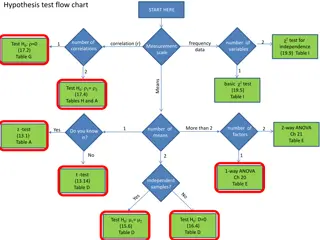
Analysis of Affymetrix Arrays Using RMA and ANOVA Model
Downloaded Affymetrix arrays were loaded into R using ReadAffy(), followed by fitting the oneway ANOVA model to the RMA processed data and adjusting p-values for false discovery rate. Significant genes were identified and their annotations searched using AmiGO.

Download Presentation

Please find below an Image/Link to download the presentation.
The content on the website is provided AS IS for your information and personal use only. It may not be sold, licensed, or shared on other websites without obtaining consent from the author. Download presentation by click this link. If you encounter any issues during the download, it is possible that the publisher has removed the file from their server.
E N D
Presentation Transcript
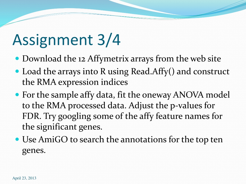
Assignment 3/4 Download the 12 Affymetrix arrays from the web site Load the arrays into R using Read.Affy() and construct the RMA expression indices For the sample affy data, fit the oneway ANOVA model to the RMA processed data. Adjust the p-values for FDR. Try googling some of the affy feature names for the significant genes. Use AmiGO to search the annotations for the top ten genes. April 23, 2013
Library(affy) rrdata <- ReadAffy() > class(rrdata) [1] "AffyBatch" attr(,"package") [1] "affy > dim(exprs(rrdata)) [1] 409600 12 > colnames(exprs(rrdata)) [1] "LN0A.CEL" "LN0B.CEL" "LN1A.CEL" "LN1B.CEL" "LN2A.CEL" "LN2B.CEL" [7] "LN3A.CEL" "LN3B.CEL" "LN4A.CEL" "LN4B.CEL" "LN5A.CEL" "LN5B.CEL" > length(probeNames(rrdata)) [1] 201800 > length(unique(probeNames(rrdata))) [1] 12625 > length((featureNames(rrdata))) [1] 12625 > featureNames(rrdata)[1:5] [1] "100_g_at" "1000_at" "1001_at" "1002_f_at" "1003_s_at" April 16, 2013 SPH 247 Statistical Analysis of Laboratory Data 2
> eset <- rma(rrdata) trying URL 'http://bioconductor.org/packages/2.1/ Content type 'application/zip' length 1352776 bytes (1.3 Mb) opened URL downloaded 1.3 Mb package 'hgu95av2cdf' successfully unpacked and MD5 sums checked The downloaded packages are in C:\Documents and Settings\dmrocke\Local Settings updating HTML package descriptions Background correcting Normalizing Calculating Expression > class(eset) [1] "ExpressionSet" attr(,"package") [1] "Biobase" > dim(exprs(eset)) [1] 12625 12 > featureNames(eset)[1:5] [1] "100_g_at" "1000_at" "1001_at" "1002_f_at" "1003_s_at" April 16, 2013 SPH 247 Statistical Analysis of Laboratory Data 3
> exprs(eset)[1:5,] LN0A.CEL LN0B.CEL LN1A.CEL LN1B.CEL LN2A.CEL LN2B.CEL LN3A.CEL 100_g_at 9.195937 9.388350 9.443115 9.012228 9.311773 9.386037 9.386089 1000_at 8.229724 7.790238 7.733320 7.864438 7.620704 7.930373 7.502759 1001_at 5.066185 5.057729 4.940588 4.839563 4.808808 5.195664 4.952883 1002_f_at 5.409422 5.472210 5.419907 5.343012 5.266068 5.442173 5.190440 1003_s_at 7.262739 7.323087 7.355976 7.221642 7.023408 7.165052 7.011527 LN3B.CEL LN4A.CEL LN4B.CEL LN5A.CEL LN5B.CEL 100_g_at 9.394606 9.602404 9.711533 9.826789 9.645565 1000_at 7.463158 7.644588 7.497006 7.618449 7.710110 1001_at 4.871329 4.875907 4.853802 4.752610 4.834317 1002_f_at 5.200380 5.436028 5.310046 5.300938 5.427841 1003_s_at 7.185894 7.235551 7.292139 7.218818 7.253799 April 16, 2013 SPH 247 Statistical Analysis of Laboratory Data 4
> summary(exprs(eset)) LN0A.CEL LN0B.CEL LN1A.CEL LN1B.CEL Min. : 2.713 Min. : 2.585 Min. : 2.611 Min. : 2.636 1st Qu.: 4.478 1st Qu.: 4.449 1st Qu.: 4.458 1st Qu.: 4.477 Median : 6.080 Median : 6.072 Median : 6.070 Median : 6.078 Mean : 6.120 Mean : 6.124 Mean : 6.120 Mean : 6.128 3rd Qu.: 7.443 3rd Qu.: 7.473 3rd Qu.: 7.467 3rd Qu.: 7.467 Max. :12.042 Max. :12.146 Max. :12.122 Max. :11.889 LN2A.CEL LN2B.CEL LN3A.CEL LN3B.CEL Min. : 2.598 Min. : 2.717 Min. : 2.633 Min. : 2.622 1st Qu.: 4.444 1st Qu.: 4.469 1st Qu.: 4.425 1st Qu.: 4.428 Median : 6.008 Median : 6.058 Median : 6.017 Median : 6.028 Mean : 6.109 Mean : 6.125 Mean : 6.116 Mean : 6.117 3rd Qu.: 7.426 3rd Qu.: 7.422 3rd Qu.: 7.444 3rd Qu.: 7.459 Max. :13.135 Max. :13.110 Max. :13.106 Max. :13.138 LN4A.CEL LN4B.CEL LN5A.CEL LN5B.CEL Min. : 2.742 Min. : 2.634 Min. : 2.615 Min. : 2.590 1st Qu.: 4.468 1st Qu.: 4.433 1st Qu.: 4.448 1st Qu.: 4.487 Median : 6.074 Median : 6.050 Median : 6.053 Median : 6.068 Mean : 6.122 Mean : 6.120 Mean : 6.121 Mean : 6.123 3rd Qu.: 7.460 3rd Qu.: 7.478 3rd Qu.: 7.477 3rd Qu.: 7.457 Max. :12.033 Max. :12.162 Max. :11.925 Max. :11.952 April 16, 2013 SPH 247 Statistical Analysis of Laboratory Data 5
> dim(exprs(eset)) [1] 12625 12 > exprs(eset)[942,] LN0A.CEL LN0B.CEL LN1A.CEL LN1B.CEL LN2A.CEL LN2B.CEL LN3A.CEL LN3B.CEL 9.063619 9.427203 9.570667 9.234590 8.285440 7.739298 8.696541 8.876506 LN4A.CEL LN4B.CEL LN5A.CEL LN5B.CEL 9.425838 9.925823 9.512081 9.426103 > group <- as.factor(c(0,0,1,1,2,2,3,3,4,4,5,5)) > group [1] 0 0 1 1 2 2 3 3 4 4 5 5 Levels: 0 1 2 3 4 5 > anova(lm(exprs(eset)[942,] ~ group)) Analysis of Variance Table Response: exprs(eset)[942, ] Df Sum Sq Mean Sq F value Pr(>F) group 5 3.7235 0.7447 10.726 0.005945 ** Residuals 6 0.4166 0.0694 --- Signif. codes: 0 *** 0.001 ** 0.01 * 0.05 . 0.1 1 April 23, 2013
> colnames(exprs(eset)) [1] "LN0A.CEL" "LN0B.CEL" "LN1A.CEL" "LN1B.CEL" "LN2A.CEL" "LN2B.CEL" [7] "LN3A.CEL" "LN3B.CEL" "LN4A.CEL" "LN4B.CEL" "LN5A.CEL" "LN5B.CEL" > group <- factor(c(0,0,1,1,2,2,3,3,4,4,5,5)) > vlist <- list(group=group) > vlist $group [1] 0 0 1 1 2 2 3 3 4 4 5 5 Levels: 0 1 2 3 4 5 > eset.lmg <- neweS(exprs(eset),vlist) > lmg.results <- LMGene(eset.lmg) This results in a list of 1173 genes that are differentially expressed after using the moderated F statistic. Compare to 119 if the moderated statistic is not used. We will see later how to understand the biological implications of the results April 23, 2013
> genediff.results <- genediff(eset.lmg) > names(genediff.results) [1] "Gene.Specific" "Posterior" > hist(genediff.results$Gene.Specific) > hist(genediff.results$Posterior) > pv2 <- pvadjust(genediff.results) > names(pv2) [1] "Gene.Specific" "Posterior" "Gene.Specific.FDR" [4] "Posterior.FDR" > sum(pv2$Gene.Specific < .05) [1] 2615 > sum(pv2$Posterior < .05) [1] 3082 > sum(pv2$Gene.Specific.FDR < .05) [1] 119 > sum(pv2$Posterior.FDR < .05) [1] 1173 Using genediff results in two lists of 12625 p-values. One uses the standard 6df denominator and the other uses the moderated F-statistic with a denominator derived from an analysis of all of the MSE s from all the linear models. April 23, 2013
> genediff.results <- genediff(eset.lmg) > class(genediff.results) [1] "list" > length(genediff.results) [1] 2 > names(genediff.results) [1] "Gene.Specific" "Posterior" > length(genediff.results$Posterior) [1] 12625 > genediff.results$Posterior[1:5] [1] 0.02939858 0.07524596 0.34409615 0.26903574 0.19198230 > sort(genediff.results$Posterior)[1:5] [1] 5.939886e-08 2.059263e-07 2.257690e-07 2.429635e-07 2.750870e-07 > order(genediff.results$Posterior)[1:5] [1] 4343 7278 12607 7030 8691 > genediff.results$Posterior[order(genediff.results$Posterior)[1:5]] [1] 5.939886e-08 2.059263e-07 2.257690e-07 2.429635e-07 2.750870e-07 April 23, 2013
> featureNames(eset.lmg)[1:5] [1] "100_g_at" "1000_at" "1001_at" "1002_f_at" "1003_s_at" > featureNames(eset.lmg)[order(genediff.results$Posterior)[1:5]] [1] "34301_r_at" "37208_at" "AFFX-M27830_5_at" "36962_at" [5] "38608_at" > featureNames(eset.lmg)[order(genediff.results$Posterior)[1:10]] [1] "34301_r_at" "37208_at" "AFFX-M27830_5_at" "36962_at" [5] "38608_at" "33646_g_at" "2027_at" "31957_r_at" [9] "34592_at" "256_s_at" Feature Gene Feature Gene 34301_r_at 33646_g_at KRT17 GM2A 37208_at 2027_at PSPH1 S100A2 AFFX-M27830_5_at 31957_r_at Endogenous control RPLP1 36962_at 34592_at COPA RPS17 38608_at 256_s_at LGALS7B RPSA April 23, 2013
For Example, RPSA 40S ribosomal protein SA GO:0006412 : translation 993 Gene Products Biological Process IEA GO:0015935 : small ribosomal subunit 89 Gene Products Cellular Component IEA GO:0003735 : structural constituent of ribosome 474 Gene Products Molecular Function IEA April 16, 2013 SPH 247 Statistical Analysis of Laboratory Data 11

")
")
[1:5,]")
)")
)")
)")
")
")
[1:5]")