Understanding Estimation and Statistical Inference in Data Analysis
Statistical inference involves acquiring information and drawing conclusions about populations from samples using estimation and hypothesis testing. Estimation determines population parameter values based on sample statistics, utilizing point and interval estimators. Interval estimates, known as confidence intervals, provide ranges within which the population parameter likely falls. Estimation is crucial in data analysis for making informed decisions and interpretations.

Download Presentation

Please find below an Image/Link to download the presentation.
The content on the website is provided AS IS for your information and personal use only. It may not be sold, licensed, or shared on other websites without obtaining consent from the author. Download presentation by click this link. If you encounter any issues during the download, it is possible that the publisher has removed the file from their server.
E N D
Presentation Transcript
Chapters 1. Introduction 2. Graphs 3. Descriptive statistics 4. Basic probability 5. Discrete distributions 6. Continuous distributions 7. Central limit theorem 8. Estimation 9. Hypothesis testing 10. Two-sample tests 13. Linear regression 14. Multivariate regression Chapter 8 Confidence Interval Estimation and Statistical Inference
Statistical Inference Statistical inference is the process by which we acquire information and draw conclusions about populations from samples. Statistics Information Data Population Sample Inference Statistic Parameter In order to do inference, we require the skills and knowledge of descriptive statistics, probability distributions, and sampling distributions. 9/18/2024 Towson University - J. Jung 10.2
Estimation There are two types of inference: estimation and hypothesis testing; estimation is introduced first. The objective of estimation is to determine the approximate value of a population parameter on the basis of a sample statistic. E.g., the sample mean ( ) is employed to estimate the population mean ( ). There are two types of estimators: Point Estimator Interval Estimator 9/18/2024 Towson University - J. Jung 10.3
Point and Interval Estimator A point estimator draws inferences about a population by estimating the value of an unknown parameter using a single value or point. We saw earlier that point probabilities in continuous distributions were virtually zero. Likewise, we d expect that the point estimator gets closer to the parameter value with an increased sample size, but point estimators don t reflect the effects of larger sample sizes. Hence, An interval estimator draws inferences about a population by estimating the value of an unknown parameter using an interval. That is we say with some ___% confidence that the population parameter of interest is between some lower and upper bounds . 9/18/2024 Towson University - J. Jung 10.4
Interval Estimator The interval is called confidence interval (C.I.). The chosen probability is called level of confidence. An interval estimate centered over a point estimate is reported at the endpoints of the range. Example: Suppose we want to estimate the mean summer income of a class of business students. For n=25 students, is calculated to be 400 $/week. point estimate C.I. level of confidence An alternative statement is: The mean income is between 380 and 420 $/week with 95% level. 9/18/2024 Towson University - J. Jung 10.5
Estimating when is known We can calculate an interval estimator from a sampling distribution, by: 1. Drawing a sample of size n from the population 2. Calculating its mean, 3. When X is normally (or approximately normally) distributed then it can be normalized: 4. And random variable Z will have a standard normal (or approximately normal) distribution!! 9/18/2024 Towson University - J. Jung 10.6
Lets start easy What is the probability of: ? 1.96 ? 1.96 = ? Now the other way around, what are the z- scores when: ?(?1 ? ?2) = 0.95 Again for: ?(?1 ? ?2) = 0.90 Hint: Use =norm.s.dist or =norm.s.inv appropriately. 9/18/2024 Towson University - J. Jung 10.7
Next steps Now we know that: ? 1.96 ? 1.96 = 0.95 We know from the CLT that: ? ?~? ?, ? We can now normalize this random variable: ? ? ? ? ? = ~? 0,1 9/18/2024 Towson University - J. Jung 10.8
Final steps Replace Z with the normalized expression: ? ? ? ? 1.96 1.96 = 0.95 ? Now do a bunch of algebra to get: + = P . 1 96 X . 1 96 . 95 n n 9/18/2024 Towson University - J. Jung 10.9
What if we hadnt started with 95% probability? With 95% probability the estimated interval was: n + = . 1 96 . 1 96 95 . P X X n With a 90% probability the interval is smaller: . 1 + = 645 . 1 645 90 . P X X n n In general, the formula is: + = 1 P X z X z / 2 / 2 n n 1 ? is called the level of confidence!! X 9/18/2024 Towson University - J. Jung 9.10
Confidence Interval with known ? Confidence interval + = 1 P x z x z / 2 / 2 n n True, but unknown parameter ? ? ? ? = ? ??/2 ?.?.. 1 ?: ? ??/2 ?, ? + ??/2 ? 9/18/2024 Towson University - J. Jung 10.11
Estimating when is known Thus, the probability that the interval: ? ? ?.?.. 1 ?= ? ??/2 ?, ? + ??/2 ? contains the population mean is 1 . This is a confidence interval estimator for The confidence interval is abbreviated as: C.I. 9/18/2024 Towson University - J. Jung 10.12
Graphically the actual location of the population mean may be here or here or possibly even here The population mean is a fixed but unknown quantity. It s incorrect to interpret the confidence interval estimate as a probability statement about . . The interval acts as the lower and upper limits of the interval estimate of the population mean. 9/18/2024 Towson University - J. Jung 10.13
Notation and Term - the probability in tails, the likelihood of a certain type of error or mistake. level of confidence = 1 is called critical value, the z score associated with half of alpha. Z 2 = e Z 2 is called margin of error, denoted by e. n Therefore, C.I. is the interval [point estimate e, point estimate + e]. 9/18/2024 Towson University - J. Jung 10.14
4 Commonly used Confidence Levels Confidence Level cut & keep handy! Table 10.1 9/18/2024 Towson University - J. Jung 10.15
Example A computer company samples demand during a sales period over 25 sales periods: 235 374 309 421 361 514 394 439 348 261 374 302 386 316 296 499 462 344 466 332 253 369 330 535 334 Its is known that the standard deviation of demand during a sales period is 75 computers. We want to estimate the mean demand of a sales period with 95% confidence in order to set inventory levels correctly. 9/18/2024 Towson University - J. Jung 10.16
Example In order to use our confidence interval estimator, we need the following pieces of data: Calculated from the data 370.16 1.96 , from Stats Tables or Excel. 75 Given n 25 therefore: So the 95% C.I. is (340.76, 399.56). Interpretation: The intervals got in this way contain in 95% of the time. 9/18/2024 Towson University - J. Jung 10.17
Confidence Interval A confidence interval either does or does not contain . The confidence level quantifies the risk. Out of 100 confidence intervals, approximately 95% would contain , while approximately 5% would not contain . 9/18/2024 Towson University - J. Jung 10.18
Confidence Interval 9/18/2024 Towson University - J. Jung 10.19
Interval Width A wide interval provides little information. For example, suppose we estimate with 95% confidence that an accountant s average starting salary is between $15,000 and $100,000. Contrast this with: a 95% confidence interval estimate of starting salaries between $42,000 and $45,000. The second estimate is much narrower, providing accounting students more precise information about starting salaries. 9/18/2024 Towson University - J. Jung 10.20
Interval Width A larger confidence level produces a w i d e r confidence interval Larger values of produce w i d e r confidence intervals Increasing the sample size decreases the width of the confidence interval while the confidence level can remain unchanged. More data provides better estimates 9/18/2024 Towson University - J. Jung 10.21
Selecting the Sample Size! We can control the width of the interval by determining the sample size necessary to produce narrow intervals. Suppose we want to estimate the mean demand to within 5 units ; i.e. we want the interval estimate to be: Since: It follows that Solve for n to get required sample size! that is, to produce a 95% confidence interval estimate of the mean ( 5 units), we need to sample 865 lead time periods (vs. the 25 data points we have currently). 9/18/2024 Towson University - J. Jung 10.22
Sample Size to Estimate a Mean The general formula for the sample size needed to estimate a population mean with an interval estimate of: Requires a sample size of at least this large: 9/18/2024 Towson University - J. Jung 10.23
Example: Margin of Error A lumber company must estimate the mean diameter of trees to determine whether or not there is sufficient lumber to harvest an area of forest. They need to estimate this to within 1 inch at a confidence level of 99%. The tree diameters are normally distributed with a standard deviation of 6 inches. How many trees need to be sampled? 9/18/2024 Towson University - J. Jung 10.24
Example Things we know: Confidence level = 99%, therefore =.01 1 We want , hence W=1. We are given that = 6. We compute That is, we will need to sample at least 239 trees to have a 99% confidence interval of 1 9/18/2024 Towson University - J. Jung 10.25
Inference with unknown variance! Previously, we estimate the population mean when the population standard deviation was known or given. When is unknown, we use its point estimator s and the z-statistic is replaced by the t-statistic, where the number of degrees of freedom v = n 1. NOTE: To use z or t , we require X-bar has NORMAL distribution. 9/18/2024 Towson University - J. Jung 10.26
Estimating when is unknown! When the population standard deviation is unknown and the population is normal, the statistic is: which is Student t distributed with v= n 1 degrees of freedom. The confidence interval estimator of is given by: 9/18/2024 Towson University - J. Jung 10.27
Estimating when is unknown Thus, the probability that the interval: ? ? ?.?.. 1 ?= ? ??/2 ?, ? + ??/2 ? contains the population mean is 1 . This is a confidence interval estimator for Use =t.inv to get the critical t scores. 9/18/2024 Towson University - J. Jung 10.28
Example A random sample of n = 83 companies resulted in average sales of $15.02 with a variance of 68.98. Please construct an interval estimator for average sales with a 95%. 9/18/2024 Towson University - J. Jung 10.29
Example From the data, we calculate: For this term =T.INV(0.025,82) and so: We are confident that 95% of similarly constructed confidence intervals contain the true population mean. 9/18/2024 Towson University - J. Jung 10.30
Reminder on using Excel To get the negative z value that has the specified probability to the left: t1=t.inv( ,n-1) T-distribution 0.45 0.4 0.35 P(T<t1)= 0.3 0.25 F(x) 0.2 0.15 0.1 0.05 0 -3 -2 -1 0 1 2 3 t1=t.inv( ,n-1) 9/18/2024 Towson University - J. Jung 8.31
Optional Material 9/18/2024 Towson University - J. Jung 10.32
Inference: Population Proportion When data are nominal, we count the number of occurrences of each value and calculate proportions. Thus, the parameter of interest in describing a population of nominal data is the population proportion . This parameter is based on the binomial experiment. x p = Recall the use of this statistic: n where p is the sample proportion: x successes in a sample size of n items. 9/18/2024 Towson University - J. Jung 10.33
Inference: Population Proportion When n and n(1 ) are both at least 5, the sampling distribution of p is approximately normal with: 1 ( , ( ~ N p ) ) n p Thus, = Z 1 ( ) n The confidence interval estimator for is given by: p Z p 1 ( 2 ) p n 9/18/2024 Towson University - J. Jung 10.34
Selecting the Sample Size The confidence interval estimator for a population proportion is: p + 1 ( ) p Z p p n 1 ( ) p Z p p n 2 2 Thus the (half) width of the interval (W) is: = 1 ( ) W Z p p n 2 Solving for n, we have: 2 1 ( p ) Z p = 2 n Towson University - J. Jung W 9/18/2024 10.35
Selecting the Sample Size For example, we want to know how many customers to survey in order to estimate the proportion of customers who prefer our brand to within 0.03 (with 95% confidence). i.e. our confidence interval after surveying will be p 0.03, that means W=0.03 Uh Oh. Since we haven t taken a sample yet, we don t have this sample proportion Substituting into the equation 2 2 1 ( p ) Z p . 1 96 1 ( p ) p = = = 2 ? n . 0 03 W 9/18/2024 Towson University - J. Jung 10.36
Selecting the Sample Size Two methods in each case we choose a value for p then solve the equation for n. Method 1 : no knowledge of even a rough value of p. This is a worst case scenario so we substitute: p= 0.50 Method 2 : we have some idea about the value of p. This is a better scenario and we substitute in our estimated p value. e.g. We draw a sample and get a p, then we can use this p to solve for n for the next sample that would give us the interval estimate with the required probability. 9/18/2024 Towson University - J. Jung 10.37
Selecting the Sample Size Method 1 : no knowledge of value of p, use 50%: Method 2 : p from last sample is, say, 20%: Thus, we can sample fewer people if we already have a reasonable estimate of the population proportion before starting. 9/18/2024 Towson University - J. Jung 10.38
Practice A Gallup Poll released stated with 95% confidence that the proportion of Marylanders supporting President Bush's proposal for revising Social Security was 56% with a margin of error of 3%. The number of persons polled was 1052. Verify this result. 9/18/2024 Towson University - J. Jung 10.39
Solution Step One: Identify the Random Variable: p Center: p=0.56 Step Two: Determine Its Distribution Standard Error: SQRT(0.56*0.44/1052)=0.0153 Shape: 0.56*1052 = 589>5, and 0.44*1052 = 463>5 ==>Normal Margin of Error: 0.56+-NORM.S.INV(0.025)*0.0153=0.56+-0.03 9/18/2024 Towson University - J. Jung 10.40
Example Extended Estimate the two values between which 99.7% of similar sample proportions might lie. 0.56+-NORM.S.INV(0.0015)*0.0153=0.56+-4.54 So the interval increased in size, because the probability that this interval covers the true population proportion is larger. 9/18/2024 Towson University - J. Jung 10.41