Understanding Hypotheses and Tests in Statistical Data Analysis
This material covers essential topics on hypotheses and tests in statistical data analysis, including defining hypotheses, critical regions, simple vs. composite hypotheses, and the goal of tests. It emphasizes the importance of critical regions in determining the validity of hypotheses and explores Fisher's perspective on testing hypotheses without alternatives.

Download Presentation

Please find below an Image/Link to download the presentation.
The content on the website is provided AS IS for your information and personal use only. It may not be sold, licensed, or shared on other websites without obtaining consent from the author. Download presentation by click this link. If you encounter any issues during the download, it is possible that the publisher has removed the file from their server.
E N D
Presentation Transcript
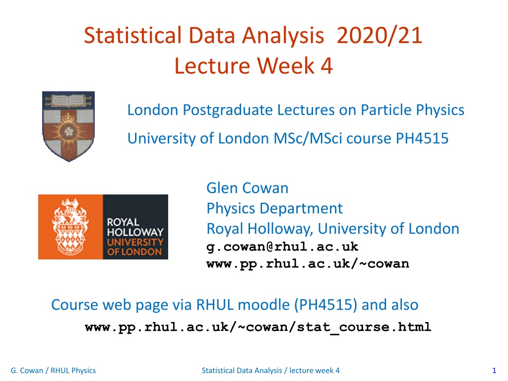
Statistical Data Analysis 2020/21 Lecture Week 4 London Postgraduate Lectures on Particle Physics University of London MSc/MSci course PH4515 Glen Cowan Physics Department Royal Holloway, University of London g.cowan@rhul.ac.uk www.pp.rhul.ac.uk/~cowan Course web page via RHUL moodle (PH4515) and also www.pp.rhul.ac.uk/~cowan/stat_course.html G. Cowan / RHUL Physics Statistical Data Analysis / lecture week 4 1
Statistical Data Analysis Lecture 4-1 Frequentist statistical tests Hypotheses Definition of a test critical region size power Type-I, Type-II errors G. Cowan / RHUL Physics Statistical Data Analysis / lecture week 4 2
Hypotheses A hypothesis Hspecifies the probability for the data, i.e., the outcome of the observation, here symbolically: x. xcould be uni-/multivariate, continuous or discrete. E.g. writex ~ P(x|H). xcould represent e.g. observation of a single object, a single event, or an entire experiment . Possible values of xform the sample space S(or data space ). Simple (or point ) hypothesis: P(x|H) completely specified. Composite hypothesis: Hcontains unspecified parameter(s). P(x|H) is also called the likelihood of the hypothesis H, often written L(H) if we want to emphasize just the dependence onH. G. Cowan / RHUL Physics Statistical Data Analysis / lecture week 4 3
Definition of a test Goal is to make some statement based on the observed data x about the validity of the possible hypotheses (here, accept or reject ). Consider a simple hypothesis H0(the null ) and an alternative H1. A test of H0is defined by specifying a critical region Wof the sample (data) space S such that there is no more than some (small) probability , assumingH0is correct, to observe the data there, i.e., P(x W | H0) is called the size of the test, prespecified equal to some small value, e.g., 0.05. S Ifxis observed in the critical region, reject H0. W G. Cowan / RHUL Physics Statistical Data Analysis / lecture week 4 4
Definition of a test (2) But in general there are an infinite number of possible critical regions that give the same size . Use the alternative hypothesisH1 to motivate where to place the critical region. Roughly speaking, place the critical region where there is a low probability ( ) to be found ifH0 is true, but high if H1 is true: G. Cowan / RHUL Physics Statistical Data Analysis / lecture week 4 5
Obvious where to put W? In the 1930s there were great debates as to the role of the alternative hypothesis. Fisher held that one could test a hypothesis H0 without reference to an alternative. Suppose, e.g., H0 predicts that x (suppose positive) usually comes out low. High values of x are less characteristic of H0, so if a high value is observed, we should reject H0, i.e., we put W at high x: If we see x here, reject H0. G. Cowan / RHUL Physics Statistical Data Analysis / lecture week 4 6
Or not so obvious where to put W? But what if the only relevant alternative to H0 is H1 as below: Here high x is more characteristic of H0 and not like what we expect from H1. So better to put W at low x. Neyman and Pearson argued that less characteristic of H0 is well defined only when taken to mean more characteristic of some relevant alternative H1 . G. Cowan / RHUL Physics Statistical Data Analysis / lecture week 4 7
Type-I, Type-II errors Rejecting the hypothesis H0 when it is true is a Type-I error. The maximum probability for this is the size of the test: P(x W | H0) But we might also accept H0 when it is false, and an alternative H1is true. This is called a Type-II error, and occurs with probability P(x S W | H1 ) = One minus this is called the power of the test with respect to the alternative H1: Power = G. Cowan / RHUL Physics Statistical Data Analysis / lecture week 4 8
Rejecting a hypothesis Note that rejecting H0 is not necessarily equivalent to the statement that we believe it is false and H1true. In frequentist statistics only associate probability with outcomes of repeatable observations (the data). In Bayesian statistics, probability of the hypothesis (degree of belief) would be found using Bayes theorem: which depends on the prior probability (H). What makes a frequentist test useful is that we can compute the probability to accept/reject a hypothesis assuming that it is true, or assuming some alternative is true. G. Cowan / RHUL Physics Statistical Data Analysis / lecture week 4 9
Statistical Data Analysis Lecture 4-2 Particle Physics example for statistical tests Statistical tests to select objects/events G. Cowan / RHUL Physics Statistical Data Analysis / lecture week 4 10
Example setting for statistical tests: the Large Hadron Collider Counter-rotating proton beams in 27 km circumference ring pp centre-of-mass energy 14 TeV Detectors at 4 pp collision points: ATLAS CMS LHCb (b physics) ALICE (heavy ion physics) general purpose G. Cowan / RHUL Physics Statistical Data Analysis / lecture week 4 11
The ATLAS detector 3000 physicists 38 countries 183 universities/labs 25 m diameter 46 m length 7000 tonnes ~108electronic channels G. Cowan / RHUL Physics Statistical Data Analysis / lecture week 4 12
A simulated SUSY event high pT jets of hadrons high pT muons p p missing transverse energy G. Cowan / RHUL Physics Statistical Data Analysis / lecture week 4 13
Background events This event from Standard Model ttbar production also has high pTjets and muons, and some missing transverse energy. can easily mimic a signal event. G. Cowan / RHUL Physics Statistical Data Analysis / lecture week 4 14
Classification viewed as a statistical test Suppose events come in two possible types: s (signal) and b (background) For each event, test hypothesis that it is background, i.e., H0 = b. Carry out test on many events, each is either of type s or b, i.e., here the hypothesis is the true class label , which varies randomly from event to event, so we can assign to it a frequentist probability. Select events for which where H0 is rejected as candidate events of type s . Equivalent Particle Physics terminology: background efficiency signal efficiency G. Cowan / RHUL Physics Statistical Data Analysis / lecture week 4 15
Example of a test for classification Suppose we can measure for each event a quantity x, where with 0 x 1. For each event in a mixture of signal (s) and background (b) test H0 : event is of type b using a critical region W of the form: W = {x : x xc}, where xcis a constant that we choose to give a test with the desired size . G. Cowan / RHUL Physics Statistical Data Analysis / lecture week 4 16
Classification example (2) Suppose we want = 10 4. Require: and therefore For this test (i.e. this critical region W), the power with respect to the signal hypothesis (s) is Note: the optimal size and power is a separate question that will depend on goals of the subsequent analysis. G. Cowan / RHUL Physics Statistical Data Analysis / lecture week 4 17
Classification example (3) Suppose that the prior probabilities for an event to be of type s or b are: s = 0.001 b = 0.999 The purity of the selected signal sample (events where b hypothesis rejected) is found using Bayes theorem: G. Cowan / RHUL Physics Statistical Data Analysis / lecture week 4 18
Classification example (4) Suppose an individual event is observed at x = 0.1. What is the probability that this event is background? (Here nothing to do with the test using x xc, just an illustration of Bayes theorem.) G. Cowan / RHUL Physics Statistical Data Analysis / lecture week 4 19
Statistical Data Analysis Lecture 4-3 Hypothesis test for classification Test statistic to define critical region Neyman-Pearson lemma G. Cowan / RHUL Physics Statistical Data Analysis / lecture week 4 20
Classifying fish You scoop up fish which are of two types: Sea Bass Cod You examine the fish with automatic sensors and for each one you measure a set of features: x1 = length x2 = width x3 = weight These constitute the feature vector x = (x1,..., xn). x4 = area of fins x5 = mean spectral reflectance x6 = ... In addition you hire a fish expert to identify the true class label y = 0 or 1 (i.e., 0 = sea bass, 1 = cod) for each fish. We thus obtain training data : (x, y)1, (x, y)2, ..., (x, y)N . G. Cowan / RHUL Physics Statistical Data Analysis / lecture week 4 21
Distributions of the features If we consider only two features x = (x1, x2), we can display the results in a scatter plot (red: y = 0, blue: y = 1). Goal is to determine a decision boundary, so that, without the help of the fish expert, we can classify new fish by seeing where their measured features lie relative to the boundary. Same idea in multi-dimensional feature space, but cannot represent as 2-D plot. Decision boundary is n-dim. hypersurface. G. Cowan / RHUL Physics Statistical Data Analysis / lecture week 4 22
Decision function, test statistic A surface in an n-dimensional space can be described by scalar function constant Different values of the constant tc result in a family of surfaces. Problem is reduced to finding the best decision function or test statistic t(x). G. Cowan / RHUL Physics Learning from data at the LHC / 8 December 2017 23
Distribution of t(x) By forming a test statistic t(x), the boundary of the critical region in the n-dimensional x-space is determined by a single single value tc. f(t|H0) f(t|H1) tc W G. Cowan / RHUL Physics Learning from data at the LHC / 8 December 2017 24
Types of decision boundaries So what is the optimal boundary for the critical region, i.e., what is the optimal test statistic t(x)? First find best t(x), later address issue of optimal size of test. Remember x-space can have many dimensions. cuts linear non-linear G. Cowan / RHUL Physics Statistical Data Analysis / lecture week 4 25
Test statistic based on likelihood ratio How can we choose a test s critical region in an optimal way ? Neyman-Pearson lemma states: For a test of H0 of size , to get the highest power with respect to the alternative H1 we need for all x in the critical region W likelihood ratio (LR) inside W and c outside, where c is a constant chosen to give a test of the desired size. Equivalently, optimal scalar test statistic is N.B. any monotonic function of this is leads to the same test. G. Cowan / RHUL Physics Statistical Data Analysis / lecture week 4 26
Proof of Neyman-Pearson Lemma Consider a critical region W and suppose the LR satisfies the criterion of the Neyman-Pearson lemma: P(x|H1)/P(x|H0) c for all x in W, P(x|H1)/P(x|H0) c for all x not in W. W Try to change this into a different critical region W retaining the same size , i.e., W+ To do so add a part W+, but to keep the size , we need to remove a part W , i.e., W W G. Cowan / RHUL Physics Statistical Data Analysis / lecture week 4 27
Proof of Neyman-Pearson Lemma (2) W+ But we are supposing the LR is higher for all x in W removed than for the x in W+ added, and therefore W W The right-hand sides are equal and therefore G. Cowan / RHUL Physics Statistical Data Analysis / lecture week 4 28
Proof of Neyman-Pearson Lemma (3) W+ We have W Note W and W+ are disjoint, and W and W are disjoint, so by Kolmogorov s 3rd axiom, W Therefore G. Cowan / RHUL Physics Statistical Data Analysis / lecture week 4 29
Proof of Neyman-Pearson Lemma (4) And therefore i.e. the deformed critical region W cannot have higher power than the original one that satisfied the LR criterion of the Neyman-Pearson lemma. G. Cowan / RHUL Physics Statistical Data Analysis / lecture week 4 30
Statistical Data Analysis Lecture 4-4 Why the Neyman-Pearson lemma usually doesn t help us Strategies for multivariate analysis Linear discriminant analysis G. Cowan / RHUL Physics Statistical Data Analysis / lecture week 4 31
Neyman-Pearson doesnt usually help We usually don t have explicit formulae for the pdfs f(x|s), f(x|b), so for a given xwe can t evaluate the likelihood ratio Instead we may have Monte Carlo models for signal and background processes, so we can produce simulated data: generate x ~ f(x|s) x1,..., xN generate x ~ f(x|b) x1,..., xN This gives samples of training data with events of known type. Can be expensive (1 fully simulated LHC event ~ 1 CPU minute). G. Cowan / RHUL Physics Statistical Data Analysis / lecture week 4 32
How is it we dont have f(x|H)? In a Monte Carlo simulation of a complex process, the fundamental hypothesis does not predict the pdf for the finally measured variables x but rather for some intermediate set of latent variables, say, z1. So in step 1 we sample z1 ~ f(z1|H), followed by many further intermediate steps: z2 ~ f(z2|z1) z3 ~ f(z3|z2) x ~ f(x|zn) So even thought H is fully defined and we can generate x according to it, the formula for f(x|H) is an enormous integral that we cannot compute: See, e.g., Kyle Cranmer, Johann Brehmer, Gilles Louppe, The frontier of simulation-based inference, arXiv:1911.01429 [stat.ML], PNAS doi.org/10.1073/pnas.1912789117 G. Cowan / RHUL Physics Statistical Data Analysis / lecture week 4 33
Approximate LR from histograms Wantt(x) = f(x|s)/f(x|b) forxhere One possibility is to generate MC data and construct histograms for both signal and background. N(x|s) N(x|s) f(x|s) Use (normalized) histogram values to approximate LR: x N(x|b) N(x|b) f(x|b) Can work well for single variable. x G. Cowan / RHUL Physics Statistical Data Analysis / lecture week 4 34
Approximate LR from 2D-histograms Suppose problem has 2 variables. Try using 2-D histograms: back- ground signal Approximate pdfs using N(x,y|s), N(x,y|b) in corresponding cells. But if we want M bins for each variable, then in n-dimensions we have Mncells; can t generate enough training data to populate. Histogram method usually not usable for n > 1 dimension. G. Cowan / RHUL Physics Statistical Data Analysis / lecture week 4 35
Strategies for multivariate analysis Neyman-Pearson lemma gives optimal answer, but cannot be used directly, because we usually don t have f(x|s), f(x|b). Histogram method with M bins for n variables requires that we estimate Mn parameters (the values of the pdfs in each cell), so this is rarely practical. A compromise solution is to assume a certain functional form for the test statistic t(x) with fewer parameters; determine them (using MC) to give best separation between signal and background. Alternatively, try to estimate the probability densities f(x|s) and f(x|b) (with something better than histograms) and use the estimated pdfs to construct an approximate likelihood ratio. G. Cowan / RHUL Physics Statistical Data Analysis / lecture week 4 36
Multivariate methods (Machine Learning) Many new (and some old) methods: Fisher discriminant Neural networks Kernel density methods Support Vector Machines Decision trees Boosting Bagging G. Cowan / RHUL Physics Statistical Data Analysis / lecture week 4 37
Resources on multivariate methods C.M. Bishop, Pattern Recognition and Machine Learning, Springer, 2006 T. Hastie, R. Tibshirani, J. Friedman, The Elements of Statistical Learning, 2nd ed., Springer, 2009 Gareth James, Daniela Witten, Trevor Hastie and Robert Tibshirani, An Introduction to Statistical Learning, Springer, 2017, faculty.marshall.usc.edu/gareth-james/ISL/ Ilya Narsky and Frank C. Porter, Statistical Analysis Techniques in Particle Physics, Wiley, 2014. 2009 G. Cowan / RHUL Physics Statistical Data Analysis / lecture week 4 38
Software Rapidly growing area of development two important resources: scikit-learn Python-based tools for Machine Learning scikit-learn.org Large user community TMVA, H cker, Stelzer, Tegenfeldt, Voss, Voss, physics/0703039 From tmva.sourceforge.net, also distributed with ROOT Variety of classifiers Good manual, widely used in HEP G. Cowan / RHUL Physics Statistical Data Analysis / lecture week 4 39
Linear test statistic Suppose there are n input variables: x = (x1,..., xn). Consider a linear function: For a given choice of the coefficients w = (w1,..., wn) we will get pdfs f(y|s) and f(y|b) : G. Cowan / RHUL Physics Statistical Data Analysis / lecture week 4 40
Linear test statistic Fisher: to get large difference between means and small widths for f(y|s) and f(y|b), maximize the difference squared of the expectation values divided by the sum of the variances: Setting J/ wi = 0 gives: , G. Cowan / RHUL Physics Statistical Data Analysis / lecture week 4 41
The Fisher discriminant The resulting coefficients widefine a Fisher discriminant. Coefficients defined up to multiplicative constant; can also add arbitrary offset, i.e., usually define test statistic as Boundaries of the test s critical region are surfaces of constant y(x), here linear (hyperplanes): G. Cowan / RHUL Physics Statistical Data Analysis / lecture week 4 42
Fisher discriminant for Gaussian data Suppose the pdfs of the input variables, f(x|s) and f(x|b), are both multivariate Gaussians with same covariance but different means: f(x|s) = Gauss( s, V) Same covariance Vij = cov[xi, xj] f(x|b) = Gauss( b, V) In this case it can be shown that the Fisher discriminant is i.e., it is a monotonic function of the likelihood ratio and thus leads to the same critical region. So in this case the Fisher discriminant provides an optimal statistical test. G. Cowan / RHUL Physics Statistical Data Analysis / lecture week 4 43
Extra slides G. Cowan / RHUL Physics Statistical Data Analysis / lecture week 4 44
Choosing a critical region To construct a test of a hypothesis H0, we can ask what are the relevant alternatives for which one would like to have a high power. Maximize power wrt H1 = maximize probability to reject H0 if H1 is true. Often such a test has a high power not only with respect to a specific point alternative but for a class of alternatives. E.g., using a measurement x ~ Gauss ( , ) we may test H0 : = 0versus the composite alternative H1 : > 0 We get the highest power with respect to any > 0by taking the critical region x xcwhere the cut-off xc is determined by the significance level such that = P(x xc| 0). G. Cowan / RHUL Physics Statistical Data Analysis / lecture week 4 45
est of = 0 vs. > 0with x ~ Gauss(,) Standard Gaussian cumulative distribution Standard Gaussian quantile G. Cowan / RHUL Physics Statistical Data Analysis / lecture week 4 46
Choice of critical region based on power (3) But we might consider < 0as well as > 0to be viable alternatives, and choose the critical region to contain both high and low x (a two-sided test). New critical region now gives reasonable power for < 0, but less power for > 0than the original one-sided test. G. Cowan / RHUL Physics Statistical Data Analysis / lecture week 4 47
No such thing as a model-independent test In general we cannot find a single critical region that gives the maximum power for all possible alternatives (no Uniformly Most Powerful test). In HEP we often try to construct a test of H0: Standard Model (or background only , etc.) such that we have a well specified false discovery rate , = Probability to reject H0 if it is true, and high power with respect to some interesting alternative, H1: SUSY, Z , etc. But there is no such thing as a model independent test. Any statistical test will inevitably have high power with respect to some alternatives and less power with respect to others. G. Cowan / RHUL Physics Statistical Data Analysis / lecture week 4 48


")


")
")
")


")


")
")
")


?")


")


")
")