Computational Learning Theory: An Overview
Computational Learning Theory explores inductive learning algorithms that generate hypotheses from training sets, emphasizing the uncertainty of generalization. The theory introduces probabilities to measure correctness and certainty, addressing challenges in learning hidden concepts. Through examples like distinguishing genders based on height, the theory highlights the importance of statistical inference and the intersection of AI, statistics, and computation. Efficient learning algorithms aim to find hypotheses closely resembling the target concept with high probability. Developed by researchers like L. G. Valiant, this theory plays a crucial role in understanding machine learning processes.
- Computational Learning Theory
- Inductive Learning
- Hypothesis Generation
- Statistical Inference
- Machine Learning

Uploaded on Sep 21, 2024 | 0 Views
Download Presentation

Please find below an Image/Link to download the presentation.
The content on the website is provided AS IS for your information and personal use only. It may not be sold, licensed, or shared on other websites without obtaining consent from the author. Download presentation by click this link. If you encounter any issues during the download, it is possible that the publisher has removed the file from their server.
E N D
Presentation Transcript
Web-Mining Agents Computational Learning Theory Prof. Dr. Ralf M ller Dr. zg r zcep Universit t zu L beck Institut f r Informationssysteme Tanya Braun (Exercise Lab) Carla P. Gomes CS4700
Computational Learning Theory (Adapted) Slides by Carla P. Gomes and Nathalie Japkowicz (Reading: R&N AIMA 3rd ed., Chapter 18.5) Carla P. Gomes CS4700
Computational Learning Theory Inductive learning: given the training set, a learning algorithm generates a hypothesis. Run hypothesis on the test set. The results say something about how good our hypothesis is. But how much do the results really tell you? Can we be certain about how the learning algorithm generalizes? We would have to see all the examples. Insight: introduce probabilities to measure degree of certainty and correctness (Valiant 1984). Carla P. Gomes CS4700
Computational Learning Theory Example: We want to use height to distinguish men and women drawing people from the same distribution for training and testing. We can never be absolutely certain that we have learned correctly our target (hidden) concept function. (E.g., there is a non-zero chance that, so far, we have only seen a sequence of bad examples) E.g., relatively tall women and relatively short men We ll see that it s generally highly unlikely to see a long series of bad examples! (under a stationarity assumption) Carla P. Gomes CS4700
Aside: flipping a coin Carla P. Gomes CS4700
Experimental data C program simulation of flips of a fair coin: Carla P. Gomes CS4700
Experimental Data Contd. With a sufficient number of flips (set of flips=example of coin bias), large outliers become quite rare. Coin example is the key to computational learning theory! Carla P. Gomes CS4700
Computational Learning Theory Intersection of AI, statistics, and theory of computation. Introduce Probably Approximately Correct Learning concerning efficient learning For our learning procedures we would like to prove that: With high probability an (efficient) learning algorithm will find a hypothesis that is approximately identical to the hidden target concept. Note the double hedging probably and approximately. Why do we need both levels of uncertainty (in general)? Carla P. Gomes CS4700 L. G. Valiant. A theory of the learnable. Commun. ACM, 27(11):1134 1142, Nov. 1984.
Probably Approximately Correct Learning Underlying principle: Seriously wrong hypotheses can be found out almost certainly (with high probability) using a small number of examples Any hypothesis that is consistent with a significantly large set of training examples is unlikely to be seriously wrong: it must be probably approximately correct. Any (efficient) algorithm that returns hypotheses that are PAC is called a PAC-learning algorithm Carla P. Gomes CS4700
Probably Approximately Correct Learning How many examples are needed to guarantee correctness? Sample complexity (# of examples to guarantee correctness) grows with the size of the Hypothesis space Stationarity assumption: Training set and test sets are drawn from the same distribution Carla P. Gomes CS4700
Notations : Error is ``true error . Different from training error True error depends on distribution D Notations: X: set of all possible examples D: distribution from which examples are drawn H: set of all possible hypotheses N: the number of examples in the training set f: the true function to be learned Assume: the true function f is in H. Error of a hypothesis h wrt f : Probability that h differs from f on a randomly picked example: error(h) = P(h(x) f(x)| x drawn from D) Exactly what we are trying to measure with our test set. Carla P. Gomes CS4700
Approximately Correct A hypothesis h is approximately correct if: error(h) , where is a given threshold, a small constant Goal: high probability, all consistent hypotheses will be approximately correct. Show that after seeing a small (poly) number of examples N, with I.e., chance of bad hypothesis, (high error but consistent with examples) is small (i.e, less than ) Carla P. Gomes CS4700
Approximately Correct : Note that error depends on distribution D Approximately correct hypotheses lie inside the -ball around f; Those hypotheses that are seriously wrong (hb Hbad) are outside the -ball, Error(hb)= P(hb(x) f(x)| x drawn from D) > , Thus the probability that the hb (a seriously wrong hypothesis) disagrees with one example is at least (definition of error). Thus the probability that the hb (a seriously wrong hypothesis) agrees with one example is no more than (1- ). So for N examples, P(hb agrees with N examples) (1- )N. Carla P. Gomes CS4700
Approximately Correct Hypothesis The probability that Hbad contains at least one consistent hypothesis is bounded by the sum of the individual probabilities. P(Hbad contains a consistent hypothesis, agreeing with all the examples) |Hbad|(1- )N |H|(1- )N hb agrees with one example is no more than (1- ). Carla P. Gomes CS4700
P(Hbad contains a consistent hypothesis) |Hbad|(1- )N |H|(1- )N Goal Bound the probability of learning a bad hypothesis below some small number . Note: The more accuracy (smaller ), and the more certainty (with smaller ) one wants, the more examples one needs. P(Hbad contains a consistent hypothesis) Sample Complexity: Number of examples to guarantee a PAC learnable function class If the learning algorithm returns a hypothesis that is consistent with this many examples, then with probability at least (1- ) the learning algorithm has an error of at most . and the hypothesis is Probably Approximately Correct.
Probably Approximately correct hypothesis h: If the probability of a small error (error(h) ) is greater than or equal to a given threshold 1 - A bound on the number of examples (sample complexity) needed to guarantee PAC: (The more accuracy (with smaller ), and the more certainty desired (with smaller ), the more examples one needs.) One seeks for (computationally) efficient learning algorithms: sample complexity N depends only polynomially from some parameter characterizing H and one gets -correct hypothesis after polynomially many steps Theoretical results apply to fairly simple learning models (e.g., decision list learning) Carla P. Gomes CS4700
: Here one assumes that H contains target function f In case f is not contained in H one talks about agnostic PAC learning. PAC Learning Similar bound derivable: Two steps: N 1/(2 2)(ln(1/ ) + ln(|H|) Sample complexity a polynomial number of examples suffices to specify a good consistent hypothesis (error(h) ) with high probability ( 1 ). Computational complexity there is an efficient algorithm for learning a consistent hypothesis from the small sample. Let s be more specific with examples. Carla P. Gomes CS4700
Example: Boolean Functions n = 2 | | 2 H Consider H the set of all Boolean function on n attributes 1 1 So the sample complexity grows as 2n ! (same as the number of all possible examples) Not PAC-Learnable! + = n (ln ln | H |) 2 ( ) N O So, any learning algorithm will do not better than a lookup table if it merely returns a hypothesis that is consistent with all known examples! Intuitively what does it say about H? Finite H required! ( : or H with finite characteristics) Carla P. Gomes CS4700
Coping With Learning Complexity 1. Force learning algorithm to look for small/simple consistent hypothesis. We considered that for Decision Tree Learning, often worst case intractable though. 2. Restrict size of hypothesis space. e.g., Decision Lists (DL) restricted form of Boolean Functions: Hypotheses correspond to a series of tests, each of which is a conjunction of literals Good news: only a poly size number of examples is required for guaranteeing PAC learning K-DL functions (maximal k conjuncts) and there are efficient algorithms for learning K-DL Carla P. Gomes CS4700
Decision Lists DLs resemble Decision Trees, but with simpler structure: Series of tests, each test a conjunction of literals; If a test succeeds, decision list specifies value to return; If test fails, processing continues with the next test in the list. Forall x: Willwait(x) <-> Patrons(x,some) or (Patrons(full) & Fri/Sat(x)) No (a) (b c) Y Y N a=Patrons(x,Some) b=patrons(x,Full) c=Fri/Sat(x) Note: if we allow arbitrarily many literals per test, decision list can express all Boolean functions. Carla P. Gomes CS4700
(d) No (a) No (b) Yes (e) Yes (f) No (i) Yes (h) Yes No a=Patrons(x,None) b=Patrons(x,Some) d=Hungry(x) e=Type(x,French) f=Type(x,Italian) g=Type(x,Thai) h=Type(x,Burger) Carla P. Gomes CS4700 i=Fri/Sat(x)
K Decision Lists Decision Lists with limited expressiveness (K-DL) at most k literals per test (a) (b c) Y Y N 2-DL K-DL is PAC learnable!!! For fixed k literals, the number of examples needed for PAC learning a K-DL function is polynomial in the number of attributes n. There are efficient algorithms for learning K-DL functions. So how do we show K-DL is PAC-learnable? Carla P. Gomes CS4700
2-DL K Decision Lists: Sample Complexity (u b) Yes (w v) No (x) No (y) Yes No 1 1 What s the size of the hypothesis space H, i.e, |K-DL(n)|? + (ln ln | H |) N K-Decision Lists set of tests: each test is a conjunct of at most k literals How many possible tests (conjuncts) of length at most k, given n attributes, conj(n,k)? + + + = 2 2 2 3 2 k n n n k | ( , | ) k 2 ( ) ( ) ( ) ( ) Conj n n O n A conjunct (or test) can appear in the list as: Yes, No, absent from list So we have at most 3 |Conj(n,k)| different K-DL lists (ignoring order) But the order of the tests (or conjuncts) in a list matters. |k-DL(n)| 3 |Conj(n,k)| |Conj(n,k)|! Carla P. Gomes CS4700
After some work (: using Stirling formula say), we get (exercise) k k = ( log ( )) O n n | ( | ) n 2 K DL 2 Recall sample complexity formula 1 - Sample Complexity of K-DL is: 1 1 + (ln ln | H |) N 1 1 + k k (ln ( log ( ))) N O n n 2 For fixed k literals, the number of examples needed for PAC learning a K-DL function is polynomial in the number of attributes n, ! 2 Efficient learning algorithm a decision list of length k can be learned in polynomial time. So K-DL is PAC learnable!!! Carla P. Gomes CS4700
Decision-List-Learning Algorithm Greedy algorithm for learning decisions lists: repeatedly finds a test that agrees with some subset of the training set; adds test to the decision list under construction and removes the corresponding examples. uses the remaining examples, until there are no examples left, for constructing the rest of the decision list. (Selection strategy not specified) Carla P. Gomes CS4700
Decision-List-Learning Algorithm Greedy algorithm for learning decisions lists: Carla P. Gomes CS4700
Decision-List-Learning Algorithm : Here algorithm with selection strategy Find smallest test set for uniformly classified subset Restaurant data. Carla P. Gomes CS4700
Examples 1. H space of Boolean functions: Not PAC Learnable, hypothesis space too big: need too many examples (sample complexity not polynomial)! 2. K-DL: PAC learnable 3. Conjunction of literals: PAC learnable : PAC-Learnability depends on the hypothesis space Sometimes using a hypothesis space different form space of target functions helps! E.g. k-term DNF (k disjuncts of conjuncts with n attributes) learnable with hypothesis space consisting of k-cnfs (conjunctions of arbitrary length with disjunctions up to length k) Carla P. Gomes CS4700
Probably Approximately Correct Learning (PAC) Learning (summary) A class of functions is said to be PAC-learnable if there exists an efficient (i.e., polynomial in size of target function, size of example instances (n), 1/ , and 1/ ) Learning algorithm such that for all functions in the class, and for all probability distributions on the function's domain, and for any values of epsilon and delta (0 < , <1), using a polynomial number of examples, the algorithm will produce a hypothesis whose error is smaller than with probability at least . The error of a hypothesis is the probability that it will differ from the target function on a random element from its domain, drawn according to the given probability distribution. Basically, this means that: there is some way to learn efficiently a "pretty good approximation of the target function. the probability is as big as you like that the error is as small as you like. Carla P. Gomes CS4700 (Of course, the tighter you make the bounds, the harder the learning algorithm is likely to have to work).
Discussion Computational Learning Theory studies the tradeoffs between the expressiveness of the hypothesis language and the complexity of learning Probably Approximately Correct learning concerns efficient learning Sample complexity --- polynomial number of examples Efficient Learning Algorithm Word of caution: PAC learning results worst case complexity results. Carla P. Gomes CS4700
Sample Complexity for Infinite Hypothesis Spaces I: VC-Dimension The PAC Learning framework has 2 disadvantages: It can lead to weak bounds Sample Complexity bound cannot be established for infinite hypothesis spaces (with functions having continuous domain/range, say) We introduce new ideas for dealing with these problems: A set of instances S is shattered by hypothesis space H iff for every dichotomy of S there exists some hypothesis in H consistent with this dichotomy. 31 Carla P. Gomes CS4700 Nathalie Japkowicz
a labeling of each member of S as positive or negative Carla P. Gomes CS4700 5
VC Dimension: Example Carla P. Gomes CS4700
Sample Complexity for Infinite Hypothesis Spaces I: VC-Dimension The Vapnik-Chervonenkis dimension, VC(H), of hypothesis space H defined over instance space X is the size of the largest finite subset of X shattered by H. If arbitrarily large finite sets of X can be shattered by H, then VC(H)= 34 Carla P. Gomes CS4700 Nathalie Japkowicz
Aside: Intuitive derivation of VC dimension How to define a natural notion of dimension on Hypothesis space H(X) = {h | h: X -> {0,1}} Dimension should be monotone So define Dimension on simple/small spaces first Aim: Define dimension for all subsets H of H(X) Simple Case (H= H(X)): dim(H) = |X| (If X infinite, then dim(H) = ) Complex case (H proper subset of H(X)): dim(H) = size of biggest simple subset of H = size of biggest subset Y of X s.t. H(Y) subset of H Observation: Dim(H) = VC(H) Making Learning less Shattering https://rjlipton.wordpress.com/2014/01/19/making-learning-less-shattering/ 35 Carla P. Gomes CS4700
VC dimension and PAC Learning PAC Learning possible by restricting hypothesis space H Leads to bias Remember: Sample complexity for PAC learning With VC dimension (also applicable for infinite spaces; Hn subclass of hypothesis parameterized by n): N >= 36 Carla P. Gomes CS4700
VC Dimension: Example 2 H = Axis parallel rectangles in R2 What is the VC dimension of H Can we PAC learn? 37 Carla P. Gomes CS4700 whesse@clarkson.edu
Learning Rectangles Consider axis parallel rectangles in the real plane Can we PAC learn it ? (1) What is the VC dimension ? Some four instances (points on the rectangle) can be shattered Shows that VC(H)>=4 38 Carla P. Gomes CS4700 whesse@clarkson.edu
Learning Rectangles Consider axis parallel rectangles in the real plane Can we PAC learn it ? (1) What is the VC dimension ? But, no five instances can be shattered + + - + + Pick the topmost, bottommost, leftmost and rightmost points and give them the label + . He fifth one gets -. Cannot be shattered. Therefore VC(H) = 4 39 Carla P. Gomes CS4700 whesse@clarkson.edu
Learning Rectangles Consider axis parallel rectangles in the real plane Can we PAC learn it ? (1) What is the VC dimension ? (2) Can we give an efficient algorithm ? 40 Carla P. Gomes CS4700 whesse@clarkson.edu
Learning Rectangles Consider axis parallel rectangles in the real plane Can we PAC learn it ? (1) What is the VC dimension ? (2) Can we give an efficient algorithm ? Find the smallest rectangle that contains the positive examples (necessarily, it will not contain any negative example, and the hypothesis is consistent). Axis parallel rectangles are efficiently PAC learnable. Exercise: What is the VC dimension of intervals on R? 41 Carla P. Gomes CS4700 whesse@clarkson.edu
The Mistake Bound Model of Learning The Mistake Bound framework is different from the PAC framework as it considers learners that receive a sequence of training examples and that predict, upon receiving each example, what its target value is. (So, it has an incremental, online-flavor ) The question asked in this setting is: How many mistakes MA will the learner A make in its predictions before it learns the target concept? This question is significant in practical settings where learning must be done while the system is in actual use. 42 Carla P. Gomes CS4700 Nathalie Japkowicz
Optimal Mistake Bounds Definition: Let C be an arbitrary nonempty concept class. The optimal mistake bound for C, denoted Opt(C), is the minimum over all possible learning algorithms A of MA(C). Opt(C)=minA Learning_Algorithms MA(C) Proposition: For any concept class C, the optimal mistake bound is bound as follows: VC(C) Opt(C) log2(|C|) 43 Carla P. Gomes CS4700 Nathalie Japkowicz


 |Hbad|(1- ε")


")


, we get")