Introduction to Stereo Reconstruction in Computer Vision
This material covers the fundamental concepts in stereo reconstruction, including the pinhole camera model, perspective projection, epipolar geometry, essential and fundamental matrices, camera calibration, homography, and projective geometry. It also discusses stereo vision and 3D reconstruction from two views, as well as camera rotation and planar scenes in computer vision. The content explores various aspects of geometry and reconstruction techniques essential for understanding computer vision applications.

Download Presentation

Please find below an Image/Link to download the presentation.
The content on the website is provided AS IS for your information and personal use only. It may not be sold, licensed, or shared on other websites without obtaining consent from the author. Download presentation by click this link. If you encounter any issues during the download, it is possible that the publisher has removed the file from their server.
E N D
Presentation Transcript
Geometry 3: Stereo Reconstruction Introduction to Computer Vision Ronen Basri Weizmann Institute of Science
Material covered Pinhole camera model, perspective projection Two view geometry, general case: Epipolar geometry, the essential matrix Camera calibration, the fundamental matrix Two view geometry, degenerate cases Homography (planes, camera rotation) A taste of projective geometry Stereo vision: 3D reconstruction from two views Multi-view geometry, reconstruction through factorization
Summary of last lecture Homography Perspective (calibrated) Perspective (uncalibrated) Orthographic ???? =0 ???? =0 ???? =0 ? ?? Form Properties One-to-one (group) Concentric epipolar lines Concentric epipolar lines Parallel epipolar lines DOFs 8(5) 8(5) 8(7) 4 Eqs/pnt 2 1 1 1 Minimal configuration 4 5+ (8,linear) 7+ (8,linear) 4 Depth No Yes, up to scale Yes, projective structure Affine structure (third view required for Euclidean structure)
Camera rotation Images obtained by rotating the camera about its optical axis are related by homography: ? ?? (? = 0) Verify that ? does not depend on ?: ? =?(?11?+?12?+?13?) ?31?+?32?+?33?, ? =?(?21?+?22?+?23?) ?31?+?32?+?33? ? =?11?+?12?+?13? ?31?+?32?+?33?, ? =?(?11?+?12?+?13?) ?31?+?32?+?33?
Planar scene For a planar scene ? ??, with ? = ? +1 ???? ? = ?? + ? and ?? + ?? + ?? = ? ?? + ?? + ?? =?? ? ?(?21?+?22?+?23?+??) ?31?+?32?+?33?+?? ? =?(?11?+?12?+?13?+??) ?31?+?32?+?33?+?? ? = ?21?+?22?+?23?+???/? ?31?+?32?+?33?+???/? ? =?11?+?12?+?13?+???/? ?31?+?32?+?33?+???/? ? =
Epipolar lines epipolar plane epipolar lines epipolar lines Baseline O O ? ??? = 0
Rectification Rectification: rotation and scaling of each camera s coordinate frame to make the epipolar lines horizontal and equi-height, by bringing the two image planes to be parallel to the baseline Rectification is achieved by applying homography to each of the two images
Rectification ?? ?? Baseline O O ? ??? ???? 1? = 0
Cyclopean coordinates Given a rectified stereo rig with baseline length ?, we place the origin at the midpoint between the camera centers. a point ?,?,? is projected to: Left image: ??=?(? ?/2) Right image: ??=?(?+?/2) , ??=?? , ??=?? ? ? ? ? Cyclopean coordinates: ? =?(??+ ??) 2(?? ??), Y =?(??+ ??) 2(?? ??), ?? ? = ?? ??
Disparity ?? ??=?? ? Disparity is inverse proportional to depth Constant disparity constant depth Larger baseline, more stable reconstruction of depth (but more occlusions, correspondence is harder) (Note that disparity is defined in a rectified rig in a cyclopean coordinate frame)
The correspondence problem Stereo matching is ill-posed: Matching ambiguity: different regions may look similar
The correspondence problem Stereo matching is ill-posed: Matching ambiguity: different regions may look similar Specular reflectance: multiple depth values
Random dot stereogram Depth is perceived from a pair of random dot images Stereo perception is based solely on local information (low level)
Compared elements for correspondence Single pixel intensities Pixel color Small window (e.g. 3 3 or 5 5), often using normalized correlation to offset gain Features and edges Mini segments
Dynamic programming Each pair of epipolar lines is compared independently Local cost, sum of unary term and binary term Unary term: cost of a single match Binary term: cost of change of disparity (occlusion) Analogous to string matching ( diff in Unix)
String matching Swing String S t r i n g Start S w i n g End
String matching Cost: #substitutions + #insertions + #deletions S t r i n g S w i n g
Stereo with dynamic programming Shortest path in a grid Diagonals: constant disparity Moving along the diagonal pay unary cost (cost of pixel match) Move sideways pay binary cost, i.e. disparity change (occlusion, right or left) Cost prefers fronto-parallel planes. Penalty is paid for tilted planes
Dynamic programming on a grid Start ???= max(?? 1,?+ ?? 1,? ?,?, ?? 1,? 1+ ?? 1,? 1 ?,?, ?? 1,? 1+ ??,? 1 ?,?) Complexity?
Probability interpretation: the Viterbi algorithm Markov chain States: discrete set of disparity ? ? ?1, ,?? = ?1(?1) ?????? 1,?(?? 1,??) ?=2 Log probabilities: product sum
Probability interpretation: the Viterbi algorithm Markov chain States: discrete set of disparity log? ?1, ,?? ? = log?1?1 (log???? + log?? 1,??? 1,??) ?=2 Maximum likelihood: minimize sum of negative logs Viterbi algorithm: equivalent to shortest path
Dynamic programming: pros and cons Advantages: Simple, efficient Achieves global optimum Generally works well Disadvantages:
Dynamic programming: pros and cons Advantages: Simple, efficient Achieves global optimum Generally works well Disadvantages: Works separately on each epipolar line, does not enforce smoothness across epipolars Prefers fronto-parallel planes Too local? (considers only immediate neighbors)
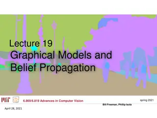
Markov random field Graph ? = ?,? In our case: graph is a 4-connected grid representing one image States: disparity Minimize energy of the form ?(?) = ??,???,?? + ??(??) (?,?) ? ? ? Interpreted as negative log probabilities
Iterated conditional modes (ICM) Initialize states (= disparities) for every pixel Update repeatedly each pixel by the most likely disparity given the values assigned to its neighbors: min ?? ??,???,?? + ??(??) ? ?(?) Markov blanket: the state of a pixel only depends on the states of its immediate neighbors Similar to Gauss-Seidel iterations Slow convergence to (often bad) local minimum
Graph cuts: expansion moves Assume ? ? is non-negative and ? ?,? is metric: ? ?,? = 0 ? ?,? = ? ?,? ? ?,? ? ?,? + ? ?,? We can apply more semi-global moves using minimal s-t cuts Converges faster to a better (local) minimum
-Expansion In any one round, expansion move allows each pixel to either change its state to , or maintain its previous state Each round is implemented via max flow/min cut One iteration: apply expansion moves sequentially with all possible disparity values Repeat till convergence
-Expansion Every round achieves a globally optimal solution over one expansion move Energy decreases (non-increasing) monotonically between rounds At convergence energy is optimal with respect to all expansion moves, and within a scale factor from the global optimum: ?(??????????) 2??(? ) where max ? ? ??(?,?) min ? ? ??(?,?) ? =
-Expansion (1D example) ? ??(?) ??(?) ????,? = 0 ?
-Expansion (1D example) ? But what about ???(??,??)? ??(??) ??(??) ?
-Expansion (1D example) ? ???(??,??) ??(??) ??(??) ?
-Expansion (1D example) ? ??(?) ???(??,?) ??(??) ?
-Expansion (1D example) ? ??(?) ???(?,??) ??(??) ?
-Expansion (1D example) ? ???(??,?) ???(?,??) ???(??,??) Such a cut cannot be obtained due to triangle inequality: ???(?,??) ?????,?? + ???(??,?) ?
Common metrics Potts model: ? ?,? = 0 ? = ? ? ? 1 ? ?,? = ? ? ? ?,? = ? ?2 Truncated 1: ? ?,? = ? ? ? ? < ? otherwise ? Truncated squared difference is not a metric
Reconstruction with graph-cuts Original Result Ground truth
A different application: detect skyline Input: one image, oriented with sky above Objective: find the skyline in the image Graph: grid Two states: sky, ground Unary (data) term: State = sky, low if blue, otherwise high State = ground, high if blue, otherwise low Binary term for vertical connections: If state(node)=sky then state(node above)=sky (infinity if not) If state(node)=ground then state(node below)= ground Solve with expansion move. This is a two state problem, and so graph cut finds the global optimum in one expansion move


")


")
")
")
")
")
")
")
")