Comprehensive Overview of Computer Vision: Topics, Techniques, and Applications
This content provides an extensive review of various topics in computer vision, ranging from image processing and 2D/3D geometry to recognition problems and machine learning basics. It covers key concepts such as filtering, edge detection, feature matching, geometric transformations, camera perspective, stereo vision, and more. Additionally, it explores topics like light perception, color, recognition techniques, and neural networks. The provided images illustrate different aspects of computer vision, serving as visual aids for better understanding.

Download Presentation

Please find below an Image/Link to download the presentation.
The content on the website is provided AS IS for your information and personal use only. It may not be sold, licensed, or shared on other websites without obtaining consent from the author. Download presentation by click this link. If you encounter any issues during the download, it is possible that the publisher has removed the file from their server.
E N D
Presentation Transcript
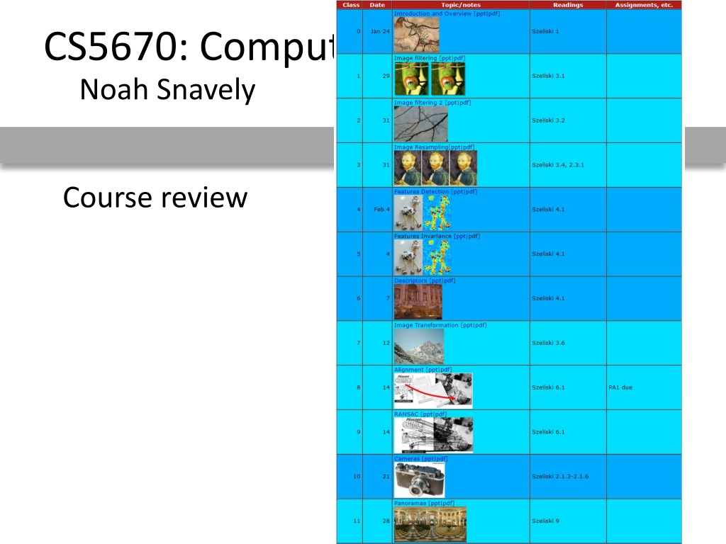
CS5670: Computer Vision Noah Snavely Course review
Topics image processing Filtering Edge detection Image resampling / aliasing / interpolation Feature detection Harris corners SIFT Invariant features Feature matching
Topics 2D geometry Image transformations Image alignment / least squares RANSAC Panoramas
Topics 3D geometry Cameras Perspective projection Single-view modeling (points, lines, vanishing points, etc.) Stereo Two-view geometry (F-matrices, E-matrices) Structure from motion Multi-view stereo
Topics geometry, continued Light, color, perception Lambertian reflectance Photometric stereo
Topics Recognition Different kinds of recognition problems Classification, detection, segmentation, etc. Machine learning basics Nearest neighbors Linear classifiers Hyperparameters Training, test, validation datasets Loss functions for classification
Topics Recognition, continued Regularization Neural networks Stochastic gradient descent Backpropagation Convolutional neural networks Architectural components: convolutional layers, pooling layers, fully connected layers Generative methods
Linear filtering One simple function on images: linear filtering (cross-correlation, convolution) Replace each pixel by a linear combination of its neighbors The prescription for the linear combination is called the kernel (or mask , filter ) 10 5 3 0 0 0 4 6 1 0 0.5 0 8 1 1 8 0 1 0.5 Local image data kernel Modified image data Source: L. Zhang
Convolution Same as cross-correlation, except that the kernel is flipped (horizontally and vertically) This is called a convolution operation: Convolution is commutative and associative
Gaussian Kernel Source: C. Rasmussen
Image gradient The gradient of an image: The gradient points in the direction of most rapid increase in intensity The edge strength is given by the gradient magnitude: The gradient direction is given by: how does this relate to the direction of the edge? Source: Steve Seitz
Finding edges gradient magnitude
Finding edges thinning (non-maximum suppression)
Image sub-sampling 1/2 1/4 (2x zoom) 1/8 (4x zoom) Why does this look so crufty? Source: S. Seitz
Subsampling with Gaussian pre-filtering Gaussian 1/2 G 1/4 G 1/8 Solution: filter the image, then subsample Source: S. Seitz
Image interpolation Ideal reconstruction Nearest-neighbor interpolation Linear interpolation Gaussian reconstruction Source: B. Curless
Image interpolation Original image: x 10 Nearest-neighbor interpolation Bilinear interpolation Bicubic interpolation
The second moment matrix The surface E(u,v) is locally approximated by a quadratic form.
The Harris operator min is a variant of the Harris operator for feature detection The trace is the sum of the diagonals, i.e., trace(H) = h11 + h22 Very similar to min but less expensive (no square root) Called the Harris Corner Detector or Harris Operator Lots of other detectors, this is one of the most popular
Laplacian of Gaussian Blob detector minima * = maximum Find maxima and minima of LoG operator in space and scale
Feature distance How to define the difference between two features f1, f2? Better approach: ratio distance = ||f1 - f2 || / || f1 - f2 || f2 is best SSD match to f1 in I2 f2 is 2nd best SSD match to f1 in I2 gives large values for ambiguous matches f2' f1 f2 I1 I2
Parametric (global) warping T p = (x,y) p = (x ,y ) Transformation T is a coordinate-changing machine: What does it mean that T is global? Is the same for any point p can be described by just a few numbers (parameters) Let s consider linear xforms (can be represented by a 2D matrix): p = T(p)
2D image transformations These transformations are a nested set of groups Closed under composition and inverse is a member
Projective Transformations aka Homographies aka Planar Perspective Maps Called a homography (or planar perspective map)
Inverse Warping Get each pixel g(x ,y ) from its corresponding location (x,y)=T-1(x,y) in f(x,y) Requires taking the inverse of the transform T-1(x,y) y y x x f(x,y) g(x ,y )
Solving for affine transformations Matrix form 6x 1 2n x 1 2n x 6
RANSAC General version: 1. Randomly choose s samples Typically s = minimum sample size that lets you fit a model 2. Fit a model (e.g., line) to those samples 3. Count the number of inliers that approximately fit the model 4. Repeat N times 5. Choose the model that has the largest set of inliers
Projecting images onto a common plane each image is warped with a homography Can t create a 360 panorama this way mosaic PP
Pinhole camera Add a barrier to block off most of the rays This reduces blurring The opening known as the aperture How does this transform the image?
Perspective Projection Projection is a matrix multiply using homogeneous coordinates: divide by third coordinate This is known as perspective projection The matrix is the projection matrix
Projection matrix intrinsics projection rotation translation (t in book s notation)
Point and line duality A line l is a homogeneous 3-vector It is to every point (ray) p on the line: lp=0 p2 p l1 p1 l l2 What is the line l spanned by rays p1 and p2 ? l is to p1 and p2 l = p1 p2 l can be interpreted as a plane normal What is the intersection of two lines l1 and l2 ? p is to l1 and l2 p = l1 l2 Points and lines are dual in projective space
Vanishing points image plane vanishing point V camera center C line on ground plane line on ground plane Properties Any two parallel lines (in 3D) have the same vanishing point v The ray from C through v is parallel to the lines An image may have more than one vanishing point in fact, every image point is a potential vanishing point
Measuring height 5.4 5 Camera height 4 3.3 3 2.8 2 1
Your basic stereo algorithm For each epipolar line For each pixel in the left image compare with every pixel on same epipolar line in right image pick pixel with minimum match cost Improvement: match windows
Stereo as energy minimization Better objective function { match cost { smoothness cost Want each pixel to find a good match in the other image Adjacent pixels should (usually) move about the same amount
Fundamental matrix epipolar line (projection of ray) epipolar line epipolar plane 0 Image 1 Image 2 This epipolar geometry of two views is described by a Very Special 3x3 matrix , called the F`undamental matrix maps (homogeneous) points in image 1 to lines in image 2! The epipolar line (in image 2) of point p is: Epipolar constraint on corresponding points:
8-point algorithm 11 f 12 f 13 f 1 u u v u u u v v v v u v 1 1 1 1 1 1 1 1 1 1 1 1 f 21 1 u u v u u u v v v v u v 2 2 2 2 2 2 2 2 2 2 2 2 = 0 f 22 f 23 1 u u v u u u v v v v u v n n n n n n n n n n n n f 31 f 32 f 33 In reality, instead of solving , we seek f to minimize , least eigenvector of . Af = Af 0 A A
Structure from motion X4 X1 X3 minimize f(R,T,P) non-linear least squares X2 X5 X7 X6 p1,1 p1,3 p1,2 Camera 1 R1,t1 Camera 3 R3,t3 Camera 2 R2,t2
Stereo: another view error depth
Radiometry What determines the brightness of an image pixel? Light source properties Sensor characteristics Surface shape Exposure Surface reflectance properties Optics Slide by L. Fei-Fei


 warping")