Input Elimination Transformations for Scalable Verification and Trace Reconstruction
This work introduces new input elimination techniques for scalable model checking in industrial applications, focusing on trace reconstruction. The transformations aim to make the netlist more tractable for solving, involving various algorithms such as retiming, phase abstraction, and bitwidth reduction. The paper also discusses the importance of consistent counterexamples, resource-intensive trace reconstruction, and the need for novel transformations to enhance model checking efficiency.

Uploaded on Sep 30, 2024 | 0 Views
Download Presentation

Please find below an Image/Link to download the presentation.
The content on the website is provided AS IS for your information and personal use only. It may not be sold, licensed, or shared on other websites without obtaining consent from the author. Download presentation by click this link. If you encounter any issues during the download, it is possible that the publisher has removed the file from their server.
E N D
Presentation Transcript
Input Elimination Transformations for Scalable Verification and Trace Reconstruction Raj Kumar Gajavelly, Jason Baumgartner, Alexander Ivrii, Robert L Kanzelman, Shiladitya Ghosh FMCAD 2019 1
Motivation: Transformation Based Verification (TBV) Design + Design + Driver + Driver + Checker Checker Trace Trace on original on original design design Reductions (transformations) are criticalfor scalable model checking in industrial applications Transform the netlist until tractable to solve Many different transformation algorithms: input elimination techniques, retiming, phase abstraction, bitwidth reduction, equivalent gate merging, localization, 140,627 registers 140,627 registers Model Checker Model Checker Combinational Combinational Optimization Optimization Engine Engine trace trace 119,147 registers 119,147 registers Counterexamples must be consistent with the original design Resource-intensive to reconstruct Semi-Formal traces on optimized design on optimized design Retiming Engine Retiming Engine trace trace 100,902 registers 100,902 registers on on optimized+retimed optimized+retimed design design We need more/new transformations Especially taking trace reconstruction into account Semi Semi- -Formal Formal Engine Engine IC3 Engine IC3 Engine In this work we present two new input elimination techniques with trivial trace reconstruction 2
Overview Motivation Contribution 1: Input Reparameterization without Logic Insertion merging inputs to constants when the changes are not observable at outputs Contribution 2: Sequentially-Unate Input Reduction merging inputs to constants while retaining existence of counterexamples Connectivity Verification Experiments Conclusion 3
Cuts A cut of the netlist is a set of nodes A cut Cdominates a node n iff every path from n to primary outputs/next-state variables goes through a node in C Two types of cuts are usually considered: min-cuts: minimum-size cuts between primary inputs and primary outputs/next-state variables dominators: single-output cuts (efficient algorithms exist for computing min-cuts and dominators) Given a cut, we consider its combinational fanin, and differentiate between Inputs dominated by the cut Registers and non-dominated gates ( cannot control these ) ( can control these ) 4
General Input Reparameterization Given a cut C, with dominated inputs Y and non-dominated gates Z 1) Compute the range of the cut in terms of Z 2) Synthesize a replacement logic producing identical range (over new inputs; at most |C| inputs are needed) 3) Replace the original logic cut with the replacement logic If |Y| > |C|, reduces input count, often also register count Reference: Baumgartner and Mony, CHARME 05 5
Fast Input Reparameterization Let F(Y, Z) define a single-output cut, with dominated inputs Y and non-dominated gates Z If for every assignment Z there exist an assignment Y0 with F(Y0, Z) = 0 and an assignment Y1 with F(Y1, Z) = 1, then F can be replaced by a new primary input Ynew A? ????:F can be replaced by a new primary input if ? ?0,?1 ( ? ?0,? ? ?1,? ) Example: Y F Ynew F Z More generally, F can be always resynthesized using a single input as ?0? (?1?) ????, where ?0? = ? ? ?,? and?1? = ? ? ?,? Reference: Een and Mishchenko, DIFTS 13 6
Input Reparameterization: Challenges Range computation can be expensive CHARME05: use BDDs to compute range of multi-output min-cuts DIFTS13: use truth-tables to compute range of 1-output, 8-input dominators MUCH faster, though lossy: can t reduce multi-output cuts Trace reconstruction can be expensive: lifting the counterexample to the original netlist is typically performed by calling a SAT-solver (on the original logic cut) to find valuation to original inputs producing the same valuation to cut gates E.g., if logic is XOR-rich and pathological for SAT solving Especially if the trace is LONG, e.g. coming from semi-formal falsification Done once per counterexample: benchmarks with many fails can be runtime-dominated by trace reconstruction Nevertheless, input reparameterization techniques yield substantial verification speedups Typically beneficial to iterate the two: maximal reductions with minimal resource Often interleaved with logic optimization, localization 7
Contribution 1: Reparameterization without Logic Insertion Idea: simplify netlist by merging inputs to constants while preserving range Let C be a cut with at least 2 dominated inputs x, Y and non-dominated gates Z If for every assignment Z every range value producible with x=1 can be also produced with x=0 (by varying values of other dominated inputs Y), then x can be merged to 0 (and similarly for merging x to 1) As 2QBF: x can be merged to 0 iff ?,? ? (? 1,?,? = ? 0, ? ,? ) x can be merged to 1 iff ?,? ? ? 0,?,? = ? 1, ? ,? 8
Examples Example 1: y1, y2 dominated, z non-dominated z z F y1 0 F y1 y2 Can merge y2 to 0 (alternatively, can merge y1 to 0) Example 2: y1, y2 dominated y1 y1 F F 0 y2 Can merge y2 to 0 (alternatively, can merge y2 to 1, or y1 to 0, or y1 to 1) Example 3: if in the above example, y1 is not dominated, then our reduction does not apply (while fast reparameterization does apply) 9
Efficient SAT-based implementation Recall: x can be merged to 0 iff 2QBF ?,? ? (? 1,?,? = ? 0, ? ,? ) is true Simple scheme: first SAT-solver enumerates range values produced with x=1; second SAT-solver checks if these range values can be also produced with x=0 Improved scheme: first SAT-solvers enumerates range values produced with x=1 such that changing x from 1 to 0 changes at least one value in the range; second SAT-solver checks if these range values can be also produced with x=0 1) Create F (1,Y,Z) copy of cut with x = 1, F (0,Y,Z) copy of cut with x = 0; enumerated = {emptyset} 2) while (!resource_exceeded) 3) if IsSAT((F F ) & !enumerated) == SAT then 4) r = assignment projected to F and Z 5) if IsSAT(F & r) == UNSAT then return Cannot Merge! r unreachable with x=0 6) else: Add r to enumerated 7) else: merge x to 0, return Merged! 10
Efficient SAT-Based Implementation: Example 1) Create F (1,Y,Z) copy of cut with x = 1, F (0,Y,Z) copy of cut with x = 0; enumerated = {emptyset} 2) while (!resource_exceeded) Cofactor dominated input x: reduction candidate 3) if IsSAT((F F ) & !enumerated) == SAT then 4) r = assignment projected to F and Z 5) if IsSAT(F & r) == UNSAT then return Cannot Merge! x y 6) Add r to enumerated Allow dominated input y to vary F z1 zn 7) else merge x to 0, return Merged! . . . Example: OR gate ? ?,?,?1, ??, with ?,? dominated inputs, ?1, ??non-dominated, to merge ? = 0 First SAT Query1: ? ? = 0,?,?1, ?? ? ? = 1,?,?1, ?? Line 3 is SAT when ?,?1, ??are all 0, r shows 1 on F due to x = 1 x = 0 Line 5 is SAT with y = 1; Line 6 add {Z = 00 & F = 1} to enumerated Repeat SAT Query2: (? ? = 0,?,?1, ?? ? ? = 1,?,?1, ??) & !{Z = 00 & F = 1} Line 3 is now UNSAT ; line 7 performs the merge with incomplete range enumeration 11
Efficient Implementation Tricks Only need to duplicate logic in fanout of x and Y. Cofactor x vs compare to original logic to simplify SAT instance 1) Create F (1,Y,Z) copy of cut with x = 1, F (0,Y,Z) copy of cut with x = 0; enumerated = {emptyset} Resource-bound by limiting #iterations, vs size of cut . Often useful to preclude analyzing cuts in fanout of previous resource-exceeded cuts; likely to also exceed resources 2) while (!resource_exceeded) 3) if IsSAT((F F ) & !enumerated) == SAT then SAT solver 1: enumerated blocked using clauses 4) r = assignment projected to F and Z SAT solver 2: r passed using assumptions 5) if IsSAT(F & r) == UNSAT then return Cannot Merge! Eagerly merge every proven-valid reduction, to ensure reduction-compatibility across candidate inputs and to accelerate later analysis. Straight-forward to parallelize 6) Add r to enumerated 7) else merge x to 0, return Merged! 12
Experimental Results: most useful cuts and parameters IBM + HWMCC benchmarks; pre-simplified without reparameterization Dom: candidate cuts are single-output dominators Dom#: # bounds number of nondominated gates Mincut: candidate cuts are min-cuts Mincut#1:#2: #1 is cut-width, #2 is #nondominated gates Mincut + Dom: dominator-based after mincut-based Interesting conclusions: Limiting #dominated inputs is not useful, unlike traditional reparameterization Smaller #s are faster, with marginally lesser reduction Dom32, 16 slowest by far Even large mincuts are much faster (next slide) Fastest maximal reductions use mincut followed by dominators Runtime (seconds) #Inputs Reduced 13
Experimental Results: Success Rate #Cuts Reduced / #Cuts Analyzed #Inputs Reduced Cuts with larger #dominated inputs vs. cut-width, and fewer nondominated gates, are more-likely reducible Processing reducible cuts first, and skipping irreducible cuts, vastly improves runtime Mincut cuwidth=4 is very fast: >90% success rate, but least input reduction Dom32 yields strong reductions, but lowest success rate and largest runtime Best reductions with fastest runtime: use faster + higher-success-rate options first, then repeat with heavier options 14
Trace Reconstruction Speedup Trace reconstruction time: our technique as preprocessing + traditional reparameterization (y axis) vs traditional reparameterization alone (x axis) Trace lifting is usually fast with traditional reparameterization, but sometimes very expensive XOR-rich logic pathological for SAT; deep counterexamples; single benchmarks with many counterexamples 29.6X faster average, up to 11808.3X faster per trace 15
Incomplete Range Computation #SAT enumerations for simple (y axis) vs improved (x axis) range computation on reducible HWMCC cuts 2.2X average reduction, up to 129.0X Much greater reduction for irreducible cuts 16
Reparameterization without Logic Insertion: Summary Simplifies netlist by merging inputs to constants Efficiently yields a subset of reparameterization reductions, without expensive range computation and trace reconstruction Often used as a lossy preprocess to reparameterization, or interleaved with: more reduction with less runtime Avoiding expensive range computations: Improved range-enumeration algorithm Use resource-constrained SAT queries of arbitrarily-large netlist cuts Not limited to small cuts as with truth-tables Often much more scalable than BDDs, especially for XOR-rich highly-controllable/dense-range cuts Use fast-and-lossy options to quickly yield most of the achievable reductions Aggressive options to yield reductions impractical with traditional reparameterization Trivial trace reconstruction: just propagate merged-to constant value for each merged input Obviate custom reduction orchestration for proving vs. bug-hunting to cope with slow trace reconstruction Enable bug-hunting to benefit from reparameterization, without trace reconstruction penalty 17
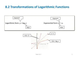
Unate Functions From literature: given a Boolean function ? ?,? x is positive unate if ? ? ? = 1,? ?(? = 0,?) x is negative unate if ? ? ? = 0,? ? ? = 1,? x is binate if neither positive nor negative unate Examples: ? ? : x is positive unate, y is negative unate ? ? : both x and y are binate Adapting this definition to combinational netlists (i.e. no registers) is easy: x is positive unate if it is positive unate with respect to every property and constraint x is negatively unate if it is negatively unate with respect to every property and constraint Theorem: in a combinational netlist If x is positive unate, then x can be merged to 1 If x is negative unate, then x can be merged to 0 Trivially-fast trace reconstruction: propagate the merged-to constant value for each merged input 18
Contribution 2: Leveraging Unateness in Sequential Netlists For sequential netlists we consider the notation of unateness based on structural analysis across registers: Let x be a primary input x is called sequentially positive unate if the number of inversions along every structural path (of any length) from x to every property and constraint is even x is called sequentially negative unate if the number of inversions along every structural path (of any length) from x to every property and constraint is odd Theorem: If x is sequentially positive unate, then x can be merged to 1 If x is sequentially negative unate, then x can be merged to 0 Again, trivially-fast trace reconstruction 19
Unateness Examples P Example 1: ?0 ?1 ?2 x x is sequentially positive unate However, x is not (combinationally) positive unate in R0 can merge x to 1 P Example 2: ?0 ?1 ?2 x x is sequentially negative unate can merge x to 0 Example 3: P ?0 ?1 ?2 x Paths from x to P exist both with an even and an odd number of inversions x is sequentially binate can t merge 20
Sequentially-Unate Input Reduction (SUR) Analysing (structurally) the polarity on each path from an input to each property, across latches/registers Linear-time algorithm; any input affecting properties/constraints in at most one polarity is sequentially-unate and reducible 1) sequentiallyUnateInputReduction(netlist N) 2) for each property and constraint gate g 3) markPolarityAIG(g, positive) 4) for each input x 5) if getPolarity(x) {positive, negative} then // x is sequentially-unate 6) merge x to (getPolarity(x) {positive}) ? constant_ONE : constant_ZERO 7) markPolarityAIG(gate g, polarity p) 8) if isInverted(g) then p p; g uninvert(g) 9) if getPolarity(g) covers p then return // already marked 10) addPolarity(g, p) 11) for each gate-input i of g 12) markPolarityAIG(i, p) 21
Verification Speedup with SUR Unate Inputs 16 18 24 6 8 684 61 93 61 3 8 40 40 8 2 2 Unate Ands 24 38 48 12 22 44545 183 711 183 3 15 48 64 15 2 2 Solving Time (sec) 12250.4 9994.1 11153.8 7627.5 1046.1 831.5 248.7 346.1 201.4 1061.9 155.6 90 95 212.9 35.8 34.9 Reduced Solving Time (sec) 2908.4 2930.4 8950.5 6917.7 647.9 673 115.9 240.2 98.9 970.5 121.1 56.4 64.5 184.6 18.8 19.6 Benchmark Inputs Ands oski2ub5i 6s429 oski4ui oski5ui 6s301 6s115 bob1u05cu mentorbm1 bob05 6s143 6s310r oski1rub03 oski1rub07 6s8 nusmvtcastp2 nusmv.tcast2.B 13231 13335 11836 3175 1048 1966 100 164 100 425 86 13074 13071 86 146 146 174682 419135 122438 24689 101655 121473 17647 24996 17647 13928 3014 109711 109665 3016 2744 2744 Sequential input reduction verification speedup: up to 4.2x and 36% average HWMCC17 Benchmarks with unate inputs Excluding some mentorbm* benchmarks having 56% average SUR inputs 22
Connectivity Verification Verifies trace bus logic, sometimes called debug bus verification Intertwined with functional logic Enables post-Si observability and performance monitoring Automated testbench creation from post-Si templates detailing observability configurations Involves creating a reference trace bus against which implementation is compared Risk subtle design instrumentation bugs: clocking / latching / power-savings problems, hierarchy-spanning compatibility problems, Often verified at full core- or chip-level to cover such problems Interaction with functional logic undermines most scalability boosts such as domain reduction 23
Connectivity Verification SUR Reductions Localization is very helpful at placing cutpoints (removing logic) without affecting provability Many of these cutpoints are sequentially unate and trigger additional reductions Reduction in Inputs Reduction in ANDs Reduction in Registers Netlist size passing into IC3 after aggressive reductions without SUR (x axis) vs with SUR (y axis) #inputs, #ANDs, #registers reduced up to 27.6x, 11.2x, 21.6x respectively 24
Connectivity Verification Reduction Speedups Comparing traditional reparameterization vs our techniques RegistersTraditional Reparam. Inputs/Time(sec) 112161 6154 / 62.3 456243 1799 / 2.2 115676 7406 / 63.2 111966 6416 / 79.3 109463 5670 / 49.7 5351515 1980356 5391085 2035734 New Input Elimination Inputs / Time (sec) 1546 / 19.1 400 / 1.5 1580 / 18.1 1547 / 19.5 1472 / 27.7 333 / 0.5 319 / 0.6 Benchmark Inputs Ands Runtime without SUR reduction (in seconds) DBV1 DBV2 DBV3 DBV4 DBV5 DBV6 DBV7 22256 21435 24111 22456 20457 24320 24168 1138339 4429287 1209308 1136918 1110112 2212 / 4.7 2219 / 12.1 SUR verification speedup Reduced Solving Time(sec) 7451.2 14037.5 8721.7 9797.1 BenchmarkLocalized Localized ANDS Localized Registers Unate Inputs Unate Ands Unate Registers Solving Time (sec) Inputs DBV1 DBV3 DBV4 DBV5 13728 16064 14395 14078 115163 157329 122873 135856 12839 15612 12664 13110 12839 11923 13486 10431 112849 156636 120279 135511 12465 14923 12591 13043 14906.1 29799.8 25213.4 10629.4 Our techniques + traditional reparameterization achieve up to 99.8% input reduction, verification runtime speedup of 13.2x Runtime with SUR reduction (in seconds) 25
Conclusions Presented two novel sound and complete input elimination transforms with trivial trace reconstruction 1) 2QBF-based input elimination, reparameterization without logic insertion Often faster than multi-output traditional reparameterization; obviates full range computation Orders of magnitude speedup to traditional reparameterization s trace reconstruction, when used as a preprocessing transform 2) Sequentially-unate input reduction Structural technique, linear runtime On classes of benchmarks e.g. connectivity verification, achieves up to 99.8% logic reduction Both are fast enough to include in generic logic optimization orchestration phase Boost scalability of end-to-end proof and bug-hunting model checking flows 26
Questions? 27

")


")