Understanding Analysis of Variance (ANOVA) in Animal Genetics & Breeding
ANOVA is a statistical method that partitions the total variance into components attributable to different factors in animal genetics and breeding. This lecture covers the concept of ANOVA, its types, application in Completely Randomized Design, calculations of Sum of Squares, and Mean Squares. It explains how ANOVA helps in experimental design by analyzing the variance due to different assignable causes, such as treatment effects and errors, in homogeneous groups of animals.
Download Presentation

Please find below an Image/Link to download the presentation.
The content on the website is provided AS IS for your information and personal use only. It may not be sold, licensed, or shared on other websites without obtaining consent from the author. Download presentation by click this link. If you encounter any issues during the download, it is possible that the publisher has removed the file from their server.
E N D
Presentation Transcript
ANIMAL GENETICS & BREEDING UNIT I Biostatistics and Computer Application Lecture 7 Analysis of Variance Dr K G Mandal Department of Animal Genetics & Breeding Bihar Veterinary College, Patna Bihar Animal Sciences University, Patna
Analysis of Variance ( ANOVA) Analysis of variance partitioning the total variance into different components of variance attributable to different assignable causes of component which is due to extraneous uncontrolled factor called error. Concept of analysis of variance was given by Prof. R. A. Fisher. Types: 1. One-way analysis 2. Two-way analysis is the technique of variation and residual
ANOVAin Completely Randomized Design (i) This design of experiment is used when the experimental units form a homogeneous group. Example: Day old chicks, Laboratory animals mice, rats, G. pigs, and animals of same age and weight, etc. (ii)Random allotment of experimental units (i.e. animals) is done with the help of lottery system or table of random numbers.
(iii) Total number of animals requiredfor the experiment or replications for each treatment is decided by error df t (n 1) = 10 and N = nxt Where, t = no. of treatments, n = no. replications per treatment N = Total number of animals (observations) Thus, for testing 5 treatments we require 3 replications in each treatment and total no. of animals, N = 5 x 3 = 15 in total.
(v) Calculation of Sum of Squares: (a) Total sum of squares (TSS) may be obtained by squaring all the observations and summing them up altogether. A correction factor (CF) may be subtracted from the total sum of squares to get the total corrected sum of squares (TCSS). The correction factor (CF) will be obtained as (GT)2/N. Where, GT is the grand total and N is total no. of observations.
(b) Sum of squares due to treatment (SST) is calculated by squaring the treatment total and summing them up. The C.F. is subtracted from the treatment sum of squares to get corrected sum of squares due to treatment. (c) Sum of squares due to error or within treatment sum of squares (SSE) may be obtained by subtracting treatment sum of squares from the total corrected sum of squares (TCSS). i.e., c = (a b)
(vi) Calculation of mean squares (variance): (a) Mean squares due to treatment (MST) may be obtained by dividing the corrected sum of squares due to treatment (SST) with df available for treatment. So, MST = ? ? ??? obtained by dividing the sum of squares due to error with the df available for the error. So, MSE = (b) Mean squares due to error (MSE) may be ??? ? ?
Calculation of Sum of Squares, Mean Squares: Suppose four feeds (treatments) are required to be compared for their effect on body weight gain of chicken from the following observations: T1 X1 X2 X3 X4 X5 X6 T2 X7 X8 X9 X10 X11 T3 X12 X13 X14 X15 T4 X16 X17 X18 X19 X20 Total: T1= T2 = T3 = T4 =
Grand Total (GT) = T1+ T2+ T3+ T4 Correction Factor (C.F.) = GT2 / N N = n1 + n2 + n3 + n4 Total sum of square (TSS) = x12 + x22 + x32 + ...+ x20(N)2 Total corrected SS (TCSS) = TSS - CF .. (i) Corrected SS due to treatment, SST, =( T1)2/n1+ ( T2)2/n2+ ( T3)2/n3+ ( T4)2/n4 CF ..(ii) Corrected SS due to error, SSE = TCSS SST . (iii)
Skeleton of ANOVA: Source of Variation Degrees of Freedom (df) Corrected sum of squares (SS) SST Corrected Mean Squares (MS) MST F Between treatment Within treatment (Error) Total t - 1 ??? ??? N - t SSE MSE N 1 TSS TMS
(vii) Calculation of F value: The calculated value of F may be obtained from the ratio MST and MSE. It is also called variance ratio. So, F = ??? ???
(viii) Test of significance: If calculated value of F is > the tabulated value of F at (t 1) and (N t) degrees of freedom at 5% level of significance then there is existence of significant difference between treatments. Alternatively, it may be concluded that there is no significant difference between the treatments.
(ix) Critical difference test: (a) If F is found to be significant at 5% or 1% level of significance for treatment & error degrees of freedom, then critical difference (CD) test is conducted by using the following formula comparing two means together at each time. CD = to ???(1 Where, to = tabulated value of t at error degrees of freedom for 5% level of significance, n1 and n2 are the number of observations under the two treatments to be compared. 1 ?1+ ?2)
(b) Means are arranged in ascending order and each possible pair is compared. (c) If the difference of any two means is greater than the CD value then they differ significantly otherwise they do not differ significantly and may be regarded as same or non-significant.
x) Use of CRD: (a) Experiment for the comparison of growth promoting ability of certain feeds on day old chicks, etc. (b) Experiment on very young lab animals e.g. mice, rats, guinea pigs for testing the effect of certain drugs or supplements, etc. xi) Advantages: (a) It is easy to design. (b) Statistical analysis of data is simple. (c) If some of the animals are dead or fail to provide data, the statistical analysis complicated. does not become
(xi) Disadvantages: (a) The design requires a homogeneous set of experimental units. (b) If the experimental units are not completely homogeneous, then the experimental error becomes enlarged and makes the treatment comparisons less efficient.
Problem 1. Following are the body weight gains of animals fed with different types of feed. The experiment is designed under CRD. Test whether different treatment (feed) has significant effect on body weight gain of animals or not. T1 T2 T3 T4 1 2 2 3 2 3 3 4 3 4 2 5 2 2 1 6 3 4 1 2 2 5 5 6 5 7 T1 = 20 n1 = 7 T2 = 14 n2 = 6 T3 = 15 n3 = 6 T4 = 36 n4 = 7
Steps involved: Step 1. Find out N (n1 + n2 + n3 + n4) Step 2. Find out GT ( x1 + x2 + x3 + + xN) Step 3. Find out CF ( GT2 / N) Step 4. Find out TSS ( x12 + x22 + x32 + + xN2) Step 5. Find out total corrected sum of squares: TCSS = TSS CF .. (i)
Step 6. Find out treatment sum of squares (SST): SST = (T1)2 + (T2)2 + (T3)2 + (T4)2 CF . (ii) Step 7. Find out Error Sum of Squares (SSE): SSE = TCSS SST .. (iii) Step 8. Prepare the ANOVA table
ANOVA in Randomized Block Design This is an improvement over CRD. This is applied when experimental units are heterogeneous. All the experimental units are grouped into different homogeneous blocks according to variability. Number of experimental units within each block are the multiple of treatments.
Allotment of treatment is not completely at random like CRD but the allotment is completely random within the homogeneous block.
Example: To study the effect of certain feed on body weight gain of day old chicks. Chicks are from different breeds say New Hampshire, Plymouth Rock, Cornish & Sussex. Total number of chicks = 80 Number of chicks in each breed (Group/Block) = 20 Number of treatment is 5. Number of Block (Group/Breed) = 4
Degrees of freedom: In RBD, each treatment is applied to one experimental unit within each block. Number of replication of each treatment is equal to number of blocks. Number of treatment = t Number of Block = b Degree of freedom for block = (b - 1) Degree of Freedom for treatment = (t 1)
Degree of freedom for error = (b -1)(t 1) Total degree of freedom = bt 1 Error DF = Total df [block df + treatment df] = (bt 1) [(b 1) + (t 1)] = bt 1 [b 1 + t 1] = bt 1 b + 1 t + 1 = bt b t + 1 = b(t 1) -1(t 1) = (b 1)(t 1)
Schematic diagram of Randomized Block Design of the aforesaid example: TREATMENT TOTAL BLOCK Feed 1 Feed 2 Feed 3 Feed 4 Feed - 5 New Hampshire Plymouth Rock 4 4 4 4 4 20 4 4 4 4 4 20 Cornish Sussex 4 4 4 4 4 4 4 4 4 4 20 20 Total 16 16 16 16 16 80
Table-1. Skeleton of ANOVA for RBD: Source of Variation Between Blocks Degrees of Freedom (DF) b - 1 Sum of Squares (SS) SSB Means Squares (MS) MSB F ??? ??? Between Treatment t - 1 SST MST ??? ??? Error (b - 1)(t 1) SSE MSE Total bt - 1 TCSS TMS
Data structure for RBD: Example: Effect of feed on body weight gain on day old chicks when chicks are from different breeds. Breed / Feed F1 F2 F3 F4 Total B1 X1 X2 X3 X4 B1 B2 X5 X6 X7 X8 B2 B3 X9 X10 X11 X12 B3 B4 X13 X14 X15 X16 B4 F1 F2 F3 F4 GT Total
Skeleton of ANOVA for RBD: Source of variation Between Blocks (Breeds) Between Treatment Error Degrees of Freedom b 1 Sum of Squares SSB Means Squares MSB F ??? ??? ??? ??? t - 1 SST MST (b 1)(t 1) SSE MSE Where, b = no. of blocks; t = no. of treatment
Grand Total (GT) = x1 + x2 + x3+ ..+ x16 Correction Factor (C.F.) = GT2 / N N = n1 + n2 + n3 + n4 Total sum of square (TSS) = x12 + x22 + x32 + ...+ x162 Total corrected SS (TCSS) = TSS - CF .. (i) Corrected SS due to Block (Breed), SSB, =( B1)2/n1+ ( B2)2/n2+ ( B3)2/n3+ ( B4)2/n4 CF ..(ii)
Corrected SS due to Feed (Treatment), SST, =( F1)2/n1+ ( F2)2/n2+ ( F3)2/n3+ ( F4)2/n4 CF ..(iii) Corrected SS due to error, SSE = TCSS SSB - SST ..(iv)
Precision: The number of blocks and number of treatments will be such that the error degrees of freedom should be at lest 10. Example: Number of treatment, t = 4 Number of block = b 10 = (b 1)x(4 -1) = (b 1)x3 or, 10 = 3b 3 or, 3b = 13 or, b = 13/3 = 4.2 or 4 Total no. of experimental units = 4x4 = 16
Merit of RBD: Most frequently used design. It is easy to design with one local control. Statistical analysis of data is simple but little bit tricky than CRD. It eliminates one assignable causes of variation among experimental units by using local control or blocking. The error DF in RBD is lesser than that of CRD due to removal of DF for blocks.
Demerit of RBD: 1. Whenthe number of treatments to be compared is large then it becomes difficult to get large blocks of homogeneous experimental units. 2. The analysis of data becomes difficult if one or more than one observation in RBD is missing. Under such condition it will be necessary to remove or omit that block.


