Understanding Biomedical Data and Markov Decision Processes
Explore the relationship between Biomedical Data and Markov Decision Processes through the analysis of genetic regulation, regulatory motifs, and the application of Hidden Markov Models (HMM) in complex computational tasks. Learn about the environment definition, Markov property, and Markov Decision Processes in the context of reinforcement learning tasks.

Download Presentation

Please find below an Image/Link to download the presentation.
The content on the website is provided AS IS for your information and personal use only. It may not be sold, licensed, or shared on other websites without obtaining consent from the author. Download presentation by click this link. If you encounter any issues during the download, it is possible that the publisher has removed the file from their server.
E N D
Presentation Transcript
Biomedical Data & Markov Decision Process Viktorija Leonova
Motivation Biomedical Data The traits of human body depend not only on the genes, but also on their regulation DNA is first transcribed into RNA (transport and mRNA) The mRNA then translated into proteins However, this proceess is regulated by gene expression In order to analyze this process, regulatory motiffs are to be found
Motivation - HMM As it is heavy computational task, it cannot be solved precisely, so a number of methods have been tried Modelling Treatment of Ischemic Heart Disease with Partially Observable Markov Decision Processes Endangered Seabird Habitat Management as a Partially Observable Markov Decision Process (Conservation Biology) BLUEPRINT Epigenome POHMM as a method of modelling
Definition of the environment <S, A, R, T> S is a set of states si, i = 1, 2, n A is a set of actions available in each of states a R is a set of rewards provided in each states Tis the set of transition probabilities Pr {st+1 = s| st, at}
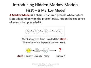
Markov Property A state that retains all relevant information is Markov, or in other words, has the Markov property. A Markov state summarizes everything important about the complete sequence of preceding state. Example: a position in checkers. Another example: A flying arrow.
Markov Environment In general case: In case of Markov environment Allows to predict all future states and rewards given only current state Provides the best possible basis for choosing actions
Markov Decision Process A reinforcement learning task that satisfies the Markov property It is finite, if the state and action spaces are finite, and the task is called finite MDP A finite MDP is defined by one-step transition probability: Pr{st+1 = s | st = s, at = a} The expected value of the next reward E {rt+1 | st = s, at = a, st+1 = s } The only information lost is the distribution of the rewards around the expected value. '= a P ss '= a ss R
Value Function Most reinforcement learning algorithms are based on estimating value functions a function of state or state-action pair, defining the advantage of being in a state or performing an action in terms of expected return Value functions are calculated for specific policies A policy is a mapping from states s S and actions a A to probability (s, a) of taking action a in state s
Value Function - continued An action value function is also defined for a given policy: Bellman s equation:
Optimal Value Functions Solving a reinforcement learning task means finding a policy that acquires sufficient reward in a long run For finite MDP it is possible to define a partial ordering of policies: is for all s S, V (s) V (s) A policy that is always better that or equal to all other policies is the optimal policy All optimal policies share unique state-value function, which is the optimal function
Optimal Value Functions They also share the same optimal state-action value function, where for all s S, all a A This function can also be expressed in terms of a value function
Methods of Solving MDP Policy iteration Value iteration Monte-Carlo methods Temporal-Difference learning
Policy Evaluation In order to evaluate a policy, we need to find its value function V (s) As per Bellman s equation, V (s) So we need to solve a set of simultaneous set of linear equations. Those can be solved iteratively, by selecting arbitrary V0(s) for all s and recursively calculating
Policy Improvement Choose arbitrary policy 0 Consider Q (s, a) for all s in turn Greedily select the action with highest Q (thus we only considering the V ) The obtained policy is better than or equal to the previous, and in the latter case it is the optimal policy Formally, =
Value Iteration In policy iteration, if policy evaluation is done iteratively, it requires a several sweeps over state set. However, the convergence to V in case of iterative can be reached only in the limit. So this process can be truncated early to save the computations. The case when policy evaluation is stopped after the first sweep is called value iteration Choose an arbitrary value V0 Update the value Vk+1(s)
Monte-Carlo Methods Monte-Carlo methods learn from experience a sample sequences of states, actions and rewards obtained from online or simulated interaction. They are based on averaging sample returns To ensure the well-defined returns, the MC methods are defined for episodic tasks. The value function can be estimated by every-visit MC, first-visit MC With a model, state values can be used to determine a policy by choosing a best combination of reward and next state
Monte-Carlo Methods: Action Values Without a model, the action values are necessary to suggest a policy Thus, the primary goal of MC methods is the estimation of Q* The method of estimation is the same with estimation state-value function Problem: many relevant state-action pairs may never be visited. If policy is deterministic, then with no returns to average, the values of some actions may never improve Maintaining exploration. Two approaches: exploring starts and stochastic policies
MC Control Alternating phases of policy evaluation and policy improvement: Example: Solving blackjack
Temporal-Difference Learning A combination of Monte-Carlo and Dynamic Programming ideas Can learn without a model Instead of Monte Carlo, need not wait until the end of the episode. For the simplest TD methods, TD(0): As it updates using the existing estimate, it is called a bootstrapping method
Temporal-Difference Methods Advantage over DP Methods: Do not need a model of the environment, its reward and probability distributions Advantage over MC methods: Naturally implemented in an online, fully-incremental fashion Prediction example: predict value of state A, given the following: MC: 0 TD: 3/4
Partially Observable MDP <S, A, T, R, , O> Where is the set of observations, and O is the set of conditional observation probabilities During a state s S an agent performs action a A, which causes the environment transition into state s S with probability T(s | s, a). At the same time, agent receives an observation o , which depends on the new state of the environment with probability O(o| s , a). Finally, the agent receives a reward R(s, a).
Partially Observable MDP As the agent does not perceive a state directly, it must make decisions under the uncertainty. In order to so, it maintains a set of beliefs. By interacting with the environment, the agent might update its beliefs by changing the probability distribution of the current state. Belief update: b = (b, a, o). As the state has Markov property, maintaining a belief over the states requires only the previous belief state, the action taken and the observation. This allows POMDP to be formulated as an MDP, where every belief is a state. The belief MDP is not partially observable anymore, since at any given time the agent knows its belief, and by extension the state of the belief MDP.
Papers Metagenomics analysis of archaeological human remains samples from Medieval Latvia as a primary screening tool for the identification of pathogen genomes. Alisa Kazarina , Guntis Gerhards, El naP tersone-Gordina, Viktorija Leonova, Ilva Pole, Valentina Capligina, Inta Jansone, and Renate Ranka