Understanding Markov Decision Processes in Machine Learning

Markov Decision Processes (MDPs) involve taking actions that influence the state of the world, leading to optimal policies. Components include states, actions, transition models, reward functions, and policies. Solving MDPs requires knowing transition models and reward functions, while reinforcement learning deals with unknown environments. Game show scenarios illustrate decision-making based on expected payoffs and optimal choices.

Download Presentation

Please find below an Image/Link to download the presentation.
The content on the website is provided AS IS for your information and personal use only. It may not be sold, licensed, or shared on other websites without obtaining consent from the author. Download presentation by click this link. If you encounter any issues during the download, it is possible that the publisher has removed the file from their server.
E N D
Presentation Transcript
CS440/ECE448 Lecture 20: Markov Decision Processes Slides by Svetlana Lazebnik, 11/2016 Modified by Mark Hasegawa-Johnson, 11/2017
Markov Decision Processes In HMMs, we see a sequence of observations and try to reason about the underlying state sequence There are no actions involved But what if we have to take an action at each step that, in turn, will affect the state of the world?
Markov Decision Processes Components that define the MDP. Depending on the problem statement, you either know these, or you learn them from data: States s, beginning with initial state s0 Actions a Each state s has actions A(s) available from it Transition model P(s | s, a) Markov assumption: the probability of going to s from s depends only on s and a and not on any other past actions or states Reward function R(s) Policy the solution to the MDP: (s) A(s): the action that an agent takes in any given state
Overview First, we will look at how to solve MDPs, or find the optimal policy when the transition model and the reward function are known Second, we will consider reinforcement learning, where we don t know the rules of the environment or the consequences of our actions
Game show A series of questions with increasing level of difficulty and increasing payoff Decision: at each step, take your earnings and quit, or go for the next question If you answer wrong, you lose everything $100 question $1,000 question $10,000 question $50,000 question Correct: $61,100 Correct Correct Correct Q1 Q2 Q3 Q4 1/2 1/100 1/10 3/4 1/2 99/100 9/10 1/4 Incorrect: $0 Incorrect: $0 Incorrect: $0 Incorrect: $0 Quit: $100 Quit: $1,100 Quit: $11,100
Game show Consider $50,000 question Probability of guessing correctly: 1/10 Quit or go for the question? What is the expected payoff for continuing? 0.1 * 61,100 + 0.9 * 0 = 6,110 What is the optimal decision? $100 question $1,000 question $10,000 question $50,000 question Correct: $61,100 Correct Correct Correct Q1 Q2 Q3 Q4 1/2 1/10 1/100 3/4 1/2 9/10 99/100 1/4 Incorrect: $0 Incorrect: $0 Incorrect: $0 Incorrect: $0 Quit: $100 Quit: $1,100 Quit: $11,100
Game show What should we do in Q3? Payoff for quitting: $1,100 Payoff for continuing: 0.5 * $11,100 = $5,550 What about Q2? $100 for quitting vs. $4,162 for continuing What about Q1? U = $3,746 U = $4,162 U = $5,550 U = $11,100 $100 question $1,000 question $10,000 question $50,000 question Correct: $61,100 Correct Correct Correct Q1 Q2 Q3 Q4 1/2 1/10 1/100 3/4 1/2 9/10 99/100 1/4 Incorrect: $0 Incorrect: $0 Incorrect: $0 Incorrect: $0 Quit: $100 Quit: $1,100 Quit: $11,100
Transition model: Grid world 0.1 0.8 0.1 R(s) = -0.04 for every non-terminal state Source: P. Abbeel and D. Klein
Goal: Policy Source: P. Abbeel and D. Klein
Grid world Transition model: R(s) = -0.04 for every non-terminal state
Grid world Optimal policy when R(s) = -0.04 for every non-terminal state
Grid world Optimal policies for other values of R(s):
Solving MDPs MDP components: States s Actions a Transition model P(s | s, a) Reward function R(s) The solution: Policy (s): mapping from states to actions How to find the optimal policy?
Maximizing expected utility The optimal policy (s) should maximize the expected utility over all possible state sequences produced by following that policy: ? ????????|?0,? = ? ?0 ? ???????? ????? ????????? ???????? ???? ?0 How to define the utility of a state sequence? Sum of rewards of individual states Problem: infinite state sequences
Utilities of state sequences Normally, we would define the utility of a state sequence as the sum of the rewards of the individual states Problem: infinite state sequences Solution: discount the individual state rewards by a factor between 0 and 1: = + + + 2 ([ , , , ]) ( ) ( ) ( ) U s s s R s R s R s 0 1 2 0 1 2 R = t = ) 1 t max ( ) 0 ( R s t 1 0 Sooner rewards count more than later rewards Makes sure the total utility stays bounded Helps algorithms converge
Utilities of states Expected utility obtained by policy starting in state s: ??? = ? ????????|?,? = ? ? ? ???????? ????? ????????? ???????? ???? ? The true utility of a state, denoted U(s), is the best possible expected sum of discounted rewards if the agent executes the best possible policy starting in state s Reminiscent of minimax values of states
Finding the utilities of states If state s has utility U(s ), then what is the expected utility of taking action a in state s? Max node s ( | ' s , ) ( ) ' s P s a U ' Chance node How do we choose the optimal action? P(s | s, a) s = * ( ) arg max s A ( | ' s , ) ( ) ' s s P s a U ( ) a ' U(s ) What is the recursive expression for U(s) in terms of the utilities of its successor states? + = max ) ( ) ( s R s U s ( | ' s , ) ( ) ' s P s a U a '
The Bellman equation Recursive relationship between the utilities of successive states: s = + ( ) ( ) max A a ( | ' s , ) ( ) ' s U s R s P s a U ( ) s ' Receive reward R(s) Choose optimal action a End up here with P(s | s, a) Get utility U(s ) (discounted by )
The Bellman equation Recursive relationship between the utilities of successive states: s = + ( ) ( ) max A a ( | ' s , ) ( ) ' s U s R s P s a U ( ) s ' For N states, we get N equations in N unknowns Solving them solves the MDP Nonlinear equations -> no closed-form solution, need to use an iterative solution method (is there a globally optimum solution?) We could try to solve them through expectiminimax search, but that would run into trouble with infinite sequences Instead, we solve them algebraically Two methods: value iteration and policy iteration
Method 1: Value iteration Start out with every U(s) = 0 Iterate until convergence During the ith iteration, update the utility of each state according to this rule: s + ( ) ( ) max A a ( | ' s , ) ( ) ' s U s R s P s a U + 1 i i ( ) s ' In the limit of infinitely many iterations, guaranteed to find the correct utility values Error decreases exponentially, so in practice, don t need an infinite number of iterations
Value iteration What effect does the update have? U s + ( ) ( ) max A a ( | ' s , ) ( ) ' s s R s P s a U + 1 i i ( ) s ' Value iteration demo
Value iteration Input (non-terminal R=-0.04) Utilities with discount factor 1 Final policy
Method 2: Policy iteration Start with some initial policy 0 and alternate between the following steps: Policy evaluation: calculate U i(s) for every state s Policy improvement: calculate a new policy i+1 based on the updated utilities Notice it s kind of like hill-climbing in the N-queens problem. Policy evaluation: Find ways in which the current policy is suboptimal Policy improvement: Fix those problems Unlike Value Iteration, this is guaranteed to converge in a finite number of steps, as long as the state space and action set are both finite.
Method 2, Step 1: Policy evaluation Given a fixed policy , calculate U (s) for every state s ' s = + ( ) ( ) ( | ' s , ( )) ( ) ' s U s R s P s s U (s) is fixed, therefore ?(? |?,? ? ) is an ? ? matrix, therefore we can solve a linear equation to get U (s)! Why is this Policy Evaluation formula so much easier to solve than the original Bellman equation? + = max ) ( ) ( a s ( | ' s , ) ( ) ' s U s R s P s a U ( ) A s '
Method 2, Step 2: Policy improvement Given U (s) for every state s, find an improved (s) s i + = 1 i ( ) arg max s A ( | ' s , ) ( ) ' s s P s a U ( ) a '
Summary MDP defined by states, actions, transition model, reward function The solution to an MDP is the policy: what do you do when you re in any given state The Bellman equation tells the utility of any given state, and incidentally, also tells you the optimum policy. The Bellman equation is N nonlinear equations in N unknowns (the policy), therefore it can t be solved in closed form. Value iteration: At the beginning of the (i+1) st iteration, each state s value is based on looking ahead i steps in time so finding the best action = optimize based on (i+1)-step lookahead Policy iteration: Find the utilities that result from the current policy, Improve the current policy