Exploring Markov Chain Random Walks in McCTRWs

Delve into the realm of Markov Chain Random Walks and McCTRWs, a method invented by a postdoc in Spain, which has shown robustness in various scenarios. Discover the premise of random walk models, the concept of IID, and its importance, along with classical problems that can be analyzed using CTRW ideas. Challenge the assumptions and foresee issues to uncover new insights in particle movements.

Download Presentation

Please find below an Image/Link to download the presentation.
The content on the website is provided AS IS for your information and personal use only. It may not be sold, licensed, or shared on other websites without obtaining consent from the author. Download presentation by click this link. If you encounter any issues during the download, it is possible that the publisher has removed the file from their server.
E N D
Presentation Transcript
+ Chapter 16 Markov Chain Random Walks McCTRWs the fast food of random walks
+Overview We are in the home stretch now and this last topic is one that is very dear to my heart as it is something that I worked very actively on myself. One of my close friends who was a postdoc in Spain at the same time as me actually invented this method and he and I have continued to work on it a lot (including that this is a core part of Nikki s PhD thesis). We have run this model in many many different problems and so far it has proven itself robust to almost any challenge we have thrown its way . What we still do not know how to do is how to parameterize it for real data from real systems.. But we re getting there.
+Basic Premise of Most Random walk Models Our particle position and time equations are given by and are random numbers. We have considered them with finite mean and variance, infinite variance and infinite mean and shown all sorts of behaviors, but we have still always assumed one thing I.I.D (Independent and Identically Distributed)
+IID Identically Distributed this means that the random number is always drawn from the same distribution. How might you relax this? Do you think it s important? In what context? Independent What do you mean by independent? Does this make sense to you How might we relax this assumption and when is it important?
+Consider the following classical problem Flow between two flat plates y x We already know from our work on Taylor dispersion how this system will behave at late times (t>L^2/D) But what about at earlier times than this? Can we use some of the CTRW ideas we have discussed to date?
+How about this? Define some distance x y x x I can measure how much time it takes particles to move this distance, right? Therefore I can say = x is fixed, t=0 and is random And now I just run my CTRW, right? And because p(t) has finite mean and variance it will converge to Fickian Dispersion (which I expect from Taylor s theory) Foresee any issues?
+Lets test it Consider the following case U=3/2 (1-y^2) -1<y<1 (parabolic flow between two plates) Let s consider x=10 (you can pick whatever you want within limits as Nikki has discovered, but lets not get sidetracked by that) Test our idea for D=0.1,0.01 and 0.001 Basically, I run a particle tracking simulation with a pulse initial condition at x=0 (represented by N particles) and then measure how long it takes each particle to travel a distance of x=10. This then gives me a vector of N travel times that I can sample from to make the next jump over x=10 (i.e. to 20) Let s test this model s ability to predict breakthrough at x=20, 40 and 100
+Step 1 Measure travel time distribution Run the code rw_ptau.m Note here that we use what is called a flux weighted initial condition (just for ease) This code runs a random walk that resolves the velocity field, i.e. In this code we store the vector, called timer, that measures the amount of time it takes each particle to cross a distance x=10. Save timer
+Step 2 Generate data for comparison Run the same random walk code that models everything too Measure BTCs at further distances rw_btcs.m Measure the amount of time it takes particles to travel a distance of 20, 40 and 100, which allows us to build brreakthrough curves btc20, btc40 and btc100.
+Step 3 - Run our Upscaled Model We now run a code that implements a CTRW and no longer resolves the velocity field, but aims to capture the different speeds of each particle by saying it takes a random time to cross a distance x. That random time is chosen from the vector timer. Sampled randomly from timer Run this code to generate arrival times/BTCs for x=20,40, 100
+Step 4 Compare the model outputs Run the code compare.m The code plot the BTCs at x=20,40 and 100 for both the fully resolved and upscaled CTRW model.
+For D=0.1 Step 1 Generate Timer
+For D=0.1 Step 2 Generate BTCs
+For D=0.1 Step 3 Run CTRW
+For D=0.1 Step 4 Compares Virtually Indistinguishable
+For D=0.01 Step 1 Generate Timer
+For D=0.01 Step 2 Generate BTCs
+For D=0.01 Step 3 Run CTRW
+For D=0.01 Step 4 Compares Not terrible But certainly Not Indistinguishable
+For D=0.001 Step 1 Generate Timer
+For D=0.001 Step 2 Generate BTCs
+For D=0.001 Step 3 Run CTRW
+For D=0.001 Step 4 Compares Seems to be getting even worse
+So what is going on? For large D the proposed CTRW model looks pretty good As D gets smaller the match between model and measured gets worse and worse WHY? What is different from the perspective of the CTRW model as D get smaller and smaller? How might you address this? And thereby improve our model so that we can match predicted and observed consistently across a range of values of D?
+What is missing? The CTRW as we have defined it assumes that successive jumps in time are completely uncorrelated and independent of one another. Our simulations suggest that this may only be true for large diffusion coefficients does this align with your intuition? As D gets smaller particles are likely to stay on similar streamlines and so it is likely that successive s will not be independent. How can mea measure and thus impose such correlation
+Travel Time Distribution x1 1 x2 2 If uncorrelated I just sample arbitrarily from p( )
+Travel Time Distribution x1 1 x2 2 Imagine I pick a specific value of 1 as shown. Now because of correlation 2 is restricted where it can come from
+Lets break p() into bins for sake of depiction say 4 x1 1 x2 2 1 2 3 4 What correlation is saying is that 2 can only come from bin 2 or 3 now and we can measure the probability that it comes from bin 2 or bin 3.
+What we have to measure x1 1 x2 2 Run a simulation with N particles (say N=one million) and for each particle measure how long it takes to cross x1 and how long it takes to cross x2 The distribution of the two should be the same Now break p(t) into M bins and attribute each particles 1 to one bin and each particles 2 to a bin. Measure how likely it is that a particle with 1 from one bin has a 1 from another one and represent it as a matrix
+Lets break p() into bins for sake of depiction say 4 x1 1 x2 2 1 2 1 2 3 3 4 4 What correlation is saying is that 2 can only come from bin 2 or 3 now and we can measure the probability that it comes from bin 2 or bin 3.
+Transition Matrix 1 2 3 4 (Next Bin) 0.8 0.2 0 0 1 How to read this 0.1 0.7 0.2 0 2 If 1 comes from bin 1 then it has an 80% chance that 2 will be from bin 1 and 20% that it will be from bin 2 and 0% chance from bins 3 or 4 0 0.15 0.75 0.1 3 0 0 0.3 0.7 4 (Initial Bin) If 1 comes from bin 3 then it has an 0% chance that 2 will be from bin 1 and 15% that it will be from bin 2, 75% from bin 3 and and 10% chance from bin 4 Thus, I randomly generate 1 from p( ). Then I generate another random number to assess where 2 will come from and then only sample from that bin. I generate a new number to assess where 3 will come from based on 2 and so on until I have jumped my desired number of steps
+Example same case as before with D=0.001 (where CTRW did not work) Recall this is what p( ) looked like If will break this into 25 bins The higher the number of bins the better you resolve correlation typically 25-50 is good.
+Check that indeed p() is the same for 1 and 2 Run code rw_ptau_2dx.m
+Measure the transition matrix Run code transition_matrix.m Bin 1 is the smallest travel times (i.e. fastest particles). Bin 25 is the largest travel times (slowest particles) 1 2
+Cumulative Transition Matrix This Matrix adds columns together last column has to be 1 Why would I do this? Easier for coding You know 1, which means you know which row you are in. To determine next bin generate a random number U=[0,1] This determines your next bin by looking along the columns..
+Now use this transition matrix to enforce correlations in a CTRW code See code mcctrw.m (sample below)
+How does this compare Recall this is what we want to reproduce
+This is what the CTRW without correlation gave us Not a good match
+How about our new algorithm Almost perfect.. Including correlation the way we have seems to fix the issues What about larger D?
+For D=0.01 What uncorrelated model gave us Better than smaller D But not Perfect
+What does transition matrix look like for our new model? Compare to smaller D
+What does transition matrix look like for our new model? D=0.001 D=0.01 What s different Does it make sense to you?
+How about our new algorithm Almost perfect.. Including correlation the way we have seems to fix the issues What about larger D?
+Finally for largest D=0.1 What uncorrelated model gave us Virtually Indistinguishable
+Transition Matrix for this Case Again, compare to before and does it make sense?
+Comparison Again, virtually perfect (but unnecessary to include correlations)
+Summary of Algorithm for McCTRW Step 1 Generate a random number from p( ) Step 2 Determine what bin is in Step 3 Generate a random number and use transition matrix to assess what the next bin will be Step 4 Generate from the new bin Step 5 - Generate a random number and use transition matrix to assess what the next bin will be Step 6 Generate from the new bin And so on until the desired number of jumps have passed.
+Ok it works for flow between two plates does it work in other flows? For this let s dig in the litterature Thursday


 into bins – for sake")

 into bins – for sake")


 is the same")