Understanding the Extension Theorem in Polynomial Mathematics
Explore the proof of the Extension Theorem, specializing in resultant calculations of polynomials and their extensions. Learn about Sylvester matrices, resultants, and how to make conjectures based on polynomial interactions. Take a deep dive into specializations and their implications in polynomial mathematics.

Download Presentation

Please find below an Image/Link to download the presentation.
The content on the website is provided AS IS for your information and personal use only. It may not be sold, licensed, or shared on other websites without obtaining consent from the author. Download presentation by click this link. If you encounter any issues during the download, it is possible that the publisher has removed the file from their server.
E N D
Presentation Transcript
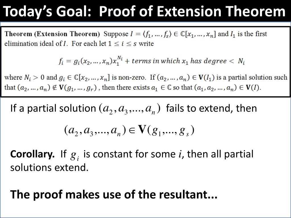
Todays Goal: Proof of Extension Theorem If a partial solution fails to extend, then ,..., , ( 3 2 a a ) n a V ( , ,..., ) ( ,..., ) a a a g g 2 3 1 n s ig is constant for some i, then all partial Corollary. If solutions extend. The proof makes use of the resultant...
Recall from last lesson... Let f and g be two polynomials in R[x] of positive degree: ) ( + = x b x b x g = + + 1 + + x 1 l l ( ) f x a x a x a x a + + 0 1 2 1 l l b + m m b 0 1 2 1 m m Syl(f, g, x)) is the matrix: Definition:The resultant of f and g with respect to x, denoted by Res(f, g, x), is the determinant of the Sylvester matrix, Res(f, g, x) = det(Syl(f, g, x)). n columns m columns Recall: Res(f, g, x) = 0 ifffandg share a common factor. Question What if one of the polynomials is a constant?
Resultants involving constant polys See Exercise 14 on page 161 of your textbook for more on this.
Time for a Game... The game is called Make a Conjecture I will present some examples; then you make a conjecture. Ready?
Example = + 2 2 ( , ) 6 ( ) 4 [ ][ ] f x y x y k y x The Sylvester matrix is a 4 x 4 square matrix. = + 2 ( , ) 3 1 [ ][ ] g x y y x x k y x Compute Res(f, g, x). 6 0 0 y y 0 6 3 = h =Res ( , , ) det f g x 0 0 2 4 0 1 3 y 2 4 1 y Res(f, g, x) is a polynomial in y; indeed, Res(f, g, x) is in the first elimination ideal f, g k[y]
Specialization 6 0 0 y y 0 6 3 = ( , , ) det f g x h(y)= Res 0 0 2 4 0 1 3 y 2 4 1 y Consider the specialization of the resultant obtained by setting y = 0. 6 0 0 0 6 3 0 0 6 3 0 = ( 3 6 ( 6 12 )) h(0) = 0 = 6 det 0 1 3 det 0 4 0 1 3 4 1 = 180 0 4 1 More generally...if then Res(f, g, x1) . ,..., , [ , 2 1 x x k g f Definition If c = (c2, c3,..., cn) kn-1 and R(x2, x3, ..., xn) := Res(f, g, x1), then a specialization of the resultant Res(f, g, x1) is R(c2, c3,..., cn). ] nx [ ,..., ] k x nx 2
Specialization Example What if we plug 0 into the polynomials at the start? = 2 ( , ) 0 6 4 f x x = + 2 2 ( , ) 6 ( ) 4 [ ][ ] f x y x y k y x = ( , ) 0 3 1 g x x = + 2 ( , ) 3 1 [ ][ ] g x y y x x k y x 6 3 0 = 30 = 0 Res( f(x, 0), g(x, 0), x) = Res(6x2 4, 3x 1) det 0 1 3 4 1 Compare this with the specialization h(0)... 6 6 0 0 0 6 3 0 0 6 3 0 = 180 h(0) = 0 6 det 0 1 3 = det 0 4 0 1 3 4 1 WHY 6? 0 4 1 We re off by a factor of 6. The 6 was zeroed out in Res( f(x, 0), g(x, 0), x) because plugging 0 into g(x, y) caused the degree of g to drop by 1.
Specialization Example Let s modify the previous example slightly... [ ) 4 ( 6 ) , ( k y x y x f + = y Setting y = 0 causes deg g to drop by 2. = 2 ( , ) 0 6 4 = + f x x 2 2 ][ ] y x = ( , ) 0 1 g x 2 ( , ) 3 1 [ ][ ] g x y y x x k y x 1 0 = 1 = Res( f(x, 0), g(x, 0), x) = Res(6x2 4, 1) det 0 1 6 0 0 y y y 0 6 3 y = h(y)= Res ( , , ) det f g x 0 0 2 4 0 1 3 y 62 2 4 1 y 6 0 0 0 0 1 0 0 6 0 0 = 36 = h(0) 62 det = det 0 1 4 0 1 0 0 4 1 More generally, if f, g k[x, y]and deg g = m with deg(g(x, 0)) = p then h(0) = LC(f)m-p Res(f(x, 0), g(x, 0), x)
Proposition 3 (Section 3.6) This result, which describes an interplay between partial solutions and resultants, will be used in the proof of the Extension Theorem...
Proof of Extension Theorem Let , where ,..., 1 s f f I = ( ) n i i x x x g f ,..., 1 2 = [ ,..., ] x x 1 n terms + N in which degree has x N i 1 i and let , a partial solution. ( ) ,..., 2 c c c n V = ( ,..., 2 c c ( ,..., , 2 1 c c ( ) I 1 ) V ( , ,..., ) g g g Want to show that if , then there exists such that . ) ) ( I c n V 1 2 n s 1c Consider the evaluation homomorphism : [ ,..., ] [ ] x x x 1 1 n defined by: = n= u = c ( ) ( , ,..., ) ( , ) f f x c c f x 1 2 1 [1x ] = The image of under is an ideal in , and is a PID. ] [1x Hence . ] ,..., I f sf 1 ( ) ( ) [ I x x 1 1
Proof of Extension Theorem We get a nice commutative diagram: [ ,..., ] x x I 1 n = ( ) ( ) I u 1x [ ] x 1 = : ) c c V ( ) { ( , }, ( ). u x f x f I I where 1 1 1 We consider two cases: Case 1: ( u Case 2: ( x u We ll use resultants to show that the second case can t actually happen. is nonconstant. , a nonzero constant. 0 u = ) 1x 1)
Proof of Extension Theorem Case 1: [ ) ( 1 x x u ] is nonconstant. 1 In this case, the FUNdamental Theorem of Algebra ensures there exists such that = c for all . 0 ) ,..., , ( 2 1 = c c f (1= c ( 2 c 1c x ) . 0 u = c ( ) { ( , : ) }, ,..., ), u x f f f I I n c Since 1 n c 1 In particular, all generators, f1, f2 , ..., fs, of I vanish at the point . ) ,..., , ( 2 1 c c ( ) ,..., ( 1 2 I c c n V n c V ( , ,..., ) ( ) c c c I Hence , so the partial solution extends, as claimed. 1 2 n )
Proof of Extension Theorem Case 2: = 0 ( u x u 1) is a nonzero constant. ) ( ,..., n g c V ( c In this case, we show leads to a contradiction. = there exists such that I f ( ) ( ,..., 2 n c c V 0 ) ,..., (2 n i c c g Now consider the resultant: , ,..., ) g g 2 1 2 s ( f = u : ) c c = ( ) { ( , }, , ( ( ,..., ) = ), u x f x f I c x n c u Since 1 1 2 c ) x 1 1 0 , ,..., ) g g g Since , there exists such that . ig 1 2 s [ ,..., ] x n x h = Res(fi, f, x1) 2
Proof of Extension Theorem = 0 ( u x u 1) is a nonzero constant. Case 2: Applying Proposition 3 to h = Res(fi, f, x1) yields: ) ( ) ( g h i c c = = 0 c deg - deg ( , ) f f x c c Res ( ( , ), ( , ), ) f x f x x 1 1 1 1 i = deg f c c ( ) Res ( ( , ), , ) g f x u x 1 0 1 i i deg if = = deg N 0 f deg f (c (c 0 ) ) g u g u i 0 i i c Hence . 0 h ( ) c , [ ,..., ] f f x x But recall: h = Res(fi, f, x1) ( ) ( = c f and 2 i n = = ( ) 0 h c ) 0 if A contradiction!


")