Microwave Filter Design Using Transmission Lines


N
o
t
e
s
2
4
ECE 5317-6351
ECE 5317-6351
Microwave Engineering
Microwave Engineering
F
a
l
l
2
0
1
9
Prof. David R. Jackson
Dept. of ECE
Filter Design Part 3:
Transmission Line Filters
1

Adapted from notes by
Prof. Jeffery T. Williams
Filter Design Using Transmission Lines
Filter Design Using Transmission Lines
2
In this set of notes we examine filter design using transmission Lines
We start with a lumped-element design.
We can use low and high impedance lines to
approximate
lumped
elements: works for
series
L
and
shunt
C
elements (what you need
in a low-pass design).
We can also apply
Richard’s transformation
to change any lumped
element design into one with transmission lines.
We can also use the
Kuroda identities
to change series TL elements
into parallel ones (more convenient for microstrip implementation).
R
e
c
i
p
e
:
3
Approximate Realization of Lumped Elements
Approximate Realization of Lumped Elements
Narrow and wide sections of microstrip line can be used to
approximately
realize
series
lumped
L
and
shunt
C
elements.
Although approximate, this is a simple technique.
This works well for
low-pass
filters (where we need series
L
and shunt
C
elements).
A
p
p
r
o
x
i
m
a
t
e
m
e
t
h
o
d
:
4
Approximate Realization of Lumped Elements (cont.)
Approximate Realization of Lumped Elements (cont.)
Consider a section of transmission line (e.g., microstrip line):
Model:
5
Approximate Realization of Lumped Elements (cont.)
Approximate Realization of Lumped Elements (cont.)
Element values in the model:
Details of calculation:
6
Approximate Realization of Lumped Elements (cont.)
Approximate Realization of Lumped Elements (cont.)
Assume:
(narrow and short microstrip line)
7
Approximate Realization of Lumped Elements (cont.)
Approximate Realization of Lumped Elements (cont.)
Assume:
(wide and short microstrip line)
8
Approximate Realization of Lumped Elements (cont.)
Approximate Realization of Lumped Elements (cont.)
From the previous derivation:
Solve for the lengths of the lines that are needed
Example
Example
9
Design an
N
= 6
Butterworth stepped-impedance low-pass filter for a matched 50
load with a cutoff frequency of 2.5 GHz
.
Choose
Z
low
= 20
,
Z
high
= 120
.
From table:
Choose type “
a
”
Example (cont.)
Example (cont.)
10
De-normalized filter:
11
Example (cont.)
Example (cont.)
Choice:
12
Example (cont.)
Example (cont.)
M
i
c
r
o
s
t
r
i
p
R
e
a
l
i
z
a
t
i
o
n
Figure 8.40 from Pozar
(not drawn to scale)
N
o
t
e
:
TX line can first be used to find the line widths (from the chosen
Z
0
values), and then used
to find the line lengths (from the calculated electrical lengths).
13
Example (cont.)
Example (cont.)
M
i
c
r
o
s
t
r
i
p
R
e
a
l
i
z
a
t
i
o
n
From p. 425 of Pozar
14
Example (cont.)
Example (cont.)
R
e
s
u
l
t
s
Figure 8.41 from Pozar
15
Example (cont.)
Example (cont.)
F
i
g
u
r
e
o
f
a
n
A
c
t
u
a
l
L
o
w
-
P
a
s
s
F
i
l
t
e
r
Richard’s Transformation
Richard’s Transformation
16
R
i
c
h
a
r
d
’
s
t
r
a
n
s
f
o
r
m
a
t
i
o
n
(
T
h
e
l
u
m
p
e
d
-
e
l
e
m
e
n
t
a
n
d
t
r
a
n
s
m
i
s
s
i
o
n
-
l
i
n
e
c
i
r
c
u
i
t
s
w
i
l
l
h
a
v
e
t
h
e
s
a
m
e
c
u
t
o
f
f
f
r
e
q
u
e
n
c
y
.
)
M
a
i
n
i
d
e
a
:
Short-circuited and open-circuited transmission lines are chosen to mimic
the performance of the lumped
L
and
C
elements, respectively.
Richard’s transformation:
=
radian frequency in lumped-element design
=
radian frequency in transmission line design
Require:
Richard’s Transformation (cont.)
Richard’s Transformation (cont.)
17
Equivalent TL model for a lumped inductor:
Require:
(same impedance property)
The inductor then has the same impedance at
any
frequency
as does the short-circuited
transmission line at corresponding frequency
.
At any frequency
, TLs can behave the same as lumped elements at frequency
.
Richard’s Transformation (cont.)
Richard’s Transformation (cont.)
18
Equivalent TL model for a lumped capacitor:
Require:
(same admittance property)
The capacitor then has the same admittance at
any
frequency
as does the open-circuited
transmission line at corresponding frequency
.
Richard’s Transformation (cont.)
Richard’s Transformation (cont.)
19
Illustration of Mapping
Kuroda’s Identities
Kuroda’s Identities
20
Kuroda’s Identity #2 is useful for transforming a series shorted TL
into a parallel open-circuited TL.
N
o
t
e
:
T
h
e
T
L
s
a
l
l
h
a
v
e
t
h
e
s
a
m
e
e
l
e
c
t
r
i
c
a
l
l
e
n
g
t
h
.
Please see the
Pozar book for a
derivation.
Example
Example
21
Design an
N
= 3
Chebyshev low-pass filter for a matched 50
load with 3.0 dB of
ripple in the passband and a cutoff frequency of 4.0 GHz
.
Choose type “
b
” low-pass prototype:
From table:
22
From table:
Final lumped-element design:
Example (cont.)
Example (cont.)
Denormalization:
Lumped elements:
23
Convert to TLs (Richard's transformation):
Example (cont.)
Example (cont.)
Recall:
24
Add extra 50
transmission lines.
Example (cont.)
Example (cont.)
These extra lines do not affect the filter performance.
25
Example (cont.)
Example (cont.)
Apply the Kuroda identity #2:
26
Example (cont.)
Example (cont.)
F
i
n
a
l
D
e
s
i
g
n
27
Example (cont.)
Example (cont.)
M
i
c
r
o
s
t
r
i
p
R
e
a
l
i
z
a
t
i
o
n
Figure 8.36 from Pozar
28
Example (cont.)
Example (cont.)
R
e
s
u
l
t
s
Figure 8.37 from Pozar
The passband
repeats with the
TL filter!
Explore the design of microwave filters using transmission lines, starting with lumped-element designs and transitioning to transmission line approximations. Learn how to realize series inductors and shunt capacitors using narrow and wide sections of microstrip lines. Discover techniques such as Richard's transformation and the Kuroda identities for effective filter design.

Download Presentation

Please find below an Image/Link to download the presentation.
The content on the website is provided AS IS for your information and personal use only. It may not be sold, licensed, or shared on other websites without obtaining consent from the author.If you encounter any issues during the download, it is possible that the publisher has removed the file from their server.
You are allowed to download the files provided on this website for personal or commercial use, subject to the condition that they are used lawfully. All files are the property of their respective owners.
The content on the website is provided AS IS for your information and personal use only. It may not be sold, licensed, or shared on other websites without obtaining consent from the author.
E N D
Presentation Transcript
Adapted from notes by Prof. Jeffery T. Williams ECE 5317-6351 Microwave Engineering Fall 2019 Prof. David R. Jackson Dept. of ECE Notes 24 Filter Design Part 3: Transmission Line Filters 1
Filter Design Using Transmission Lines In this set of notes we examine filter design using transmission Lines Recipe: We start with a lumped-element design. We can use low and high impedance lines to approximate lumped elements: works for series L and shunt C elements (what you need in a low-pass design). We can also apply Richard s transformation to change any lumped element design into one with transmission lines. We can also use the Kuroda identities to change series TL elements into parallel ones (more convenient for microstrip implementation). 2
Approximate Realization of Lumped Elements Approximate method: Narrow and wide sections of microstrip line can be used to approximately realize series lumped L and shunt C elements. Although approximate, this is a simple technique. This works well for low-pass filters (where we need series L and shunt C elements). 3
Approximate Realization of Lumped Elements (cont.) Consider a section of transmission line (e.g., microstrip line): Z 0, l ( ) ( ) = = 0cot = = Z Z jZ l 0/sin Z Z jZ l 11 22 21 12 Model: Z Z Z Z 22 21 11 21 Z 21 4
Approximate Realization of Lumped Elements (cont.) Element values in the model: Details of calculation: ( ) ( ) ( ) ( ) = 0tan / 2 Z Z jZ l = cot 1/sin Z Z jZ l l 11 21 11 21 0 ( ) l cos sin 1 l ( ) = jZ = 0/sin Z jZ l ( / 2 ) 0 21 ( ) = tan jZ l 0 1 cos sin x ( ) = Note: tan / 2 x x ( ) ( ) 0tan / 2 jZ l 0tan / 2 jZ l ( ) 0/sin jZ l 5
Approximate Realization of Lumped Elements (cont.) Assume: (narrow and short microstrip line) 1, 1 Z l 0 ( ) ( ) 0tan / 2 jZ l 0tan / 2 jZ l ( ) 0/sin jZ l ( ) = L Z l 0 ( ) jZ l 0 L Series inductor 6
Approximate Realization of Lumped Elements (cont.) Assume: 1, 1 Z l (wide and short microstrip line) 0 ( ) ( ) 0tan / 2 jZ l 0tan / 2 jZ l ( ) 0/sin jZ l 1 C ( ) = / Z l 0 C ( ) 0/ jZ l Shunt capacitor 7
Approximate Realization of Lumped Elements (cont.) From the previous derivation: ( ) = high L Z l 0 Solve for the lengths of the lines that are needed 1 C ( ) = low / Z l 0 = Choose: c ( ) = Series inductors: L Z l c high c 1 ( ) = Shunt capacitors: / Z l low C c c L ( ) = Narrow lines (series inductors): c l Z c high CZ ( ) = Wide lines (shunt capacitors): l c low c 8
Example Design an N= 6 Butterworth stepped-impedance low-pass filter for a matched 50 load with a cutoff frequency of 2.5 GHz. ChooseZlow= 20 , Zhigh= 120 . L L L R = 1 2n 4n 6n 0 R = 1 +- L C C C 5n 1n 3n Choose type a = = = = = = = = = = = = 0.517 1.414 1.932 1.932 1.414 0.517 g g g g g g C L C L C L 1 1 n From table: 2 2 n 3 3 n 4 4 n 5 5 n 6 6 n 9
Example (cont.) De-normalized filter: 2 L 4 L 6 L R = 50 0 R = 50 +- L C C C 3 5 1 = = = = = = 0.658 pF C = = = = = = 0.517 [F] 1.414 [H] 1.932 [F] 1.932 [H] 1.414 [F] 0.517 [H] C L C L C L 1 1 n 4.5 nH L 2 ( ( ) R 2 n = = / L L R 2.46 pF C 0 n c 3 3 n ) 6.15 nH L / / C C 4 4 n 0 n c 1.80 pF C 5 5 n 1.65 nH L 6 n 6 10
Example (cont.) 2 L 4 L 6 L R = 50 0 R = 50 +- L C C C 3 5 1 Choice: = = 20 120 Z Z ( ( ( ( ( ( ) ) ) ) ) ) low ( ( ( ( ( ( ) ) ) ) ) ) = = = = = = 0.658 pF C = o 0.207 rad 11.8 l 1 1 high 4.5 nH L = o 0.589 rad 11.8 l 2 2 2.46 pF C L ( ) ( ) 3 = = o 0.773 rad 44.3 #2, #4, #6 l l c 3 6.15 nH Z L c 4 high CZ = o 0.805 rad 46.1 l ( ) ( ) = 1.80 pF C #1, #3, #5 l 4 5 c low c = o 0.565 rad 32.4 l 1.65 nH L 5 6 = o 0.215 rad 12.3 l 6 11
Example (cont.) Microstrip Realization #1 #5 #3 #2 #4 #6 20 120 (not drawn to scale) Figure 8.40 from Pozar Note: TX line can first be used to find the line widths (from the chosen Z0 values), and then used to find the line lengths (from the calculated electrical lengths). 12
Example (cont.) Microstrip Realization = = = 1.58 mm , 4.2, tan 0.02 h r From p. 425 of Pozar 13
Example (cont.) Results Full wave The dotted line shows the result with substrate loss. Figure 8.41 from Pozar 14
Example (cont.) Figure of an Actual Low-Pass Filter 15
Richards Transformation Richard s transformation Main idea: Short-circuited and open-circuited transmission lines are chosen to mimic the performance of the lumped L and C elements, respectively. Richard s transformation: ( ) ( ) ( ) = tan tan l l c c =radian frequency in lumped-element design = radian frequency in transmission line design ( ) ( ) = Require: ( ) = tan 1 l = /8 @ l c c c g c (The lumped-element and transmission-line circuits will have the same cutoff frequency.) 16
Richards Transformation (cont.) At any frequency , TLs can behave the same as lumped elements at frequency . Equivalent TL model for a lumped inductor: Z Short L 0 /8 @ g c ( ) j L = Require: 0tan jZ l (same impedance property) ( ) ( ) = tan 0ta n j l L jZ l c The inductor then has the same impedance at any frequency as does the short-circuited transmission line at corresponding frequency . = Z L 0 c 17
Richards Transformation (cont.) Equivalent TL model for a lumped capacitor: = 1/ Y Z Open C 0 0 /8 @ g c ( ) j C = Require: 0tan jY l (same admittance property) ( ) ( ) = tan 0ta n j l C jY l c The capacitor then has the same admittance at any frequency as does the open-circuited transmission line at corresponding frequency . = Y C 0 c 18
Richards Transformation (cont.) Illustration of Mapping ( ) ( ) ( ) = tan tan l l c c Transmission line 2 c c Lumped element 0 c ( ) = = @ : tan 1 l l c 4 ( ) = = @2 : tan l l c 2 19
Kurodas Identities Kuroda s Identity #2 is useful for transforming a series shorted TL into a parallel open-circuited TL. Note: The TLs all have the same electrical length. Line with parallel open stub l Z Z 01 03 l Z Z 04 02 l = = 2 Z n Z l 03 01 2 Z n Z Line with series shorted stub 04 02 where Please see the Pozar book for a derivation. Z Z = + 2 1 n 02 01 20
Example Design an N= 3 Chebyshev low-pass filter for a matched 50 load with 3.0 dB of ripple in the passband and a cutoff frequency of 4.0 GHz. Choose type b low-pass prototype: N = = odd = 3 g 1 4 = = g L g L = = 1 g R 1 1n 3 3n 0 0 = = 1 S g G +- 4 Ln = g C 2 2n From table: = = = = 3.3487 0.7117 3.3487 g g g L C L 1 1 n = = 2 2 n 3 3 n 21
Example (cont.) Final lumped-element design: ( ) = 4 10 9 2 rad/s c 1L 3 L R = 50 0 R = 50 +- L C 2 From table: Denormalization: Lumped elements: = = = = = = 3.3487 H L 6.66 nH L ( ( ) R = = / L L R 1 n 1 0 n c 0.7117 F C 0.566 pF C ) 2 n / / C C 2 0 n c 3.3487 H L 6.66 nH L 3 n 3 22
Example (cont.) Convert to TLs (Richard's transformation): 70.3 = = = = 167.4 Z L 01 1 c ( L ) = 1/ Z C 02 2 c = 167.4 Z 03 3 c l l Z Z 03 01 ( ) = 4 10 9 2 rad/s c R = 50 0 R = 50 +- L Z = 1/ Z Y Recall: 02 02 02 ( ( ) l = Z L inductor 0 c = / 4 @4 GHz l ) = Y C capacitor 0 c 23
Example (cont.) Add extra 50 transmission lines. l l Z Z 03 01 1L 3 L R = 50 l l 0 R = 50 = 50 Z = 50 Z +- L 00 00 Z 02 l = / 4 @4 GHz l These extra lines do not affect the filter performance. 24
Example (cont.) Apply the Kuroda identity #2: = / 4 @4 GHz l = R = Note: Z Z 50 l 03 01 0 l R = 50 = = 2 2 Z n Z Z n Z +- L 04 01 04 03 Z Z Z 05 02 05 l l l = = 2 Z n Z Z Z 04 01 = + = 2 1 1.299 n 00 2 Z n Z 03 05 00 25
Example (cont.) Final Design = / 4 @4 GHz l R = 50 l 0 l R = 50 Z Z +- L 04 04 Z Z Z 05 02 05 l l l = = = 70.3 Z 02 217.5 Z 04 64.9 Z 05 26
Example (cont.) Microstrip Realization Figure 8.36 from Pozar 27
Example (cont.) Results 3 dB cf 2 cf The passband repeats with the TL filter! = = attenuation IL S dB 21dB Figure 8.37 from Pozar 28


")
")
")
")
")

")
")
")
")
")
")

")
")
")


")
")
")
")
")
")
")