Building Regression Model for LPGA Golf Performance - 2008
The regression model for LPGA Golf Performance in 2008 focuses on predicting prize winnings per round based on various golf performance metrics. The process includes data description, modeling strategies, selecting predictors, training the model, and assessing its validity. The analysis involves influential observations, testing model assumptions, and predicting errors. Notable golfers from the sample are listed, and the backward elimination method is demonstrated with steps and results.

Download Presentation

Please find below an Image/Link to download the presentation.
The content on the website is provided AS IS for your information and personal use only. It may not be sold, licensed, or shared on other websites without obtaining consent from the author. Download presentation by click this link. If you encounter any issues during the download, it is possible that the publisher has removed the file from their server.
E N D
Presentation Transcript
Regression Model Building LPGA Golf Performance - 2008
Data Description Response: log(Prize Winnings/Round) Skewed data Potential Predictors: Average Drive Distance Percentage of Drives Reaching Fairway Percentage of Greens Reached in Regulation Average Putts per Hole Average Number of Sand Traps Hit per Round (Sandshot) Percentage of Sand Saves Samples: Training Sample 100 Randomly Sampled Golfers Validation Sample 57 Remaining Golfers used to assess fit
Modeling Strategies Select Training Sample Select best subset of predictors based on Backward Elimination, Forward Selection, Stepwise Regression and/or All Possible Regressions based on Minimizing: ( ) ( ) log Model log( ) 2 ' AIC n SSE n n = + = ' # parameters in model p p Identify any Influential Observations (based on Outliers, Leverage Values, DFFITS, DFBETAS, Cook s D) Test Model Assumptions: Normality (Shapiro-Wilk), Constant Variance (Brown-Forsyth and Breusch-Pagan) Determine Validity of model by obtaining prediction errors for validation sample
Top of Entire Sample (First 20 Golfers) golfer Ahn, Shi Hyun Alfredsson, Helen Ammaccapane, Dina Bader, Beth Bae, Kyeong Baena, Marisa Bastel, Emily Blasberg, Erica Blomqvist, Minea Bowie Young, Heather Bunch, Ashli Burks, Audra Burton, Brandie Castrale, Nicole Cavalleri, Silvia Cho, Irene Choi, Hye Jung Choi, Na Yeon Chung, Ilmi Coutu, Taylor drive fairway green putts sandshot sandsave prz 55 49 37 73 66 66 59 44 70 58 35 28 47 61 53 49 73 55 75 37 logprz 249.4 253.8 246.3 249.1 244.0 254.2 237.4 245.4 253.2 251.0 246.6 239.2 244.2 245.2 240.7 243.5 242.5 257.4 242.6 241.0 64.6 62.7 70.2 64.1 62.4 64.7 73.6 69.2 62.6 67.4 70.1 68.6 65.5 71.3 69.1 70.2 69.3 68.5 64.6 70.0 61.2 68.2 64.6 61.2 60.7 60.9 60.5 63.2 59.7 63.0 64.7 60.5 67.3 67.1 59.6 63.3 60.9 68.5 63.0 63.0 27.44 29.36 30.20 29.78 28.38 29.21 30.60 28.68 27.35 28.83 31.36 30.11 30.62 28.92 30.08 29.29 27.78 28.43 28.54 30.13 34.5 38.8 40.5 41.1 43.9 33.3 28.8 27.3 44.3 34.5 42.9 39.3 27.7 27.9 35.8 42.9 37.0 45.5 29.3 48.6 6063 19343 1873 1212 2555 2282 921 1923 6726 2689 1281 1460 1668 7209 1947 3214 3470 14808 2827 2252 8.7099 9.8701 7.5353 7.1004 7.8459 7.7327 6.8258 7.5614 8.8137 7.8969 7.1551 7.2863 7.4193 8.8830 7.5742 8.0754 8.1518 9.6029 7.9470 7.7194
Backward Elimination (RSS = SSE) Step 1: Start: AIC=-200.22 logprz ~ drive + fairway + green + putts + sandshot + sandsave Step 2: AIC=-202.13 logprz ~ drive + green + putts + sandshot + sandsave Df Sum of Sq RSS AIC <none> 11.750 -202.132 - sandsave 1 0.400 12.150 -200.784 - drive 1 0.537 12.287 -199.665 - sandshot 1 1.034 12.784 -195.698 - green 1 32.091 43.841 -72.461 - putts 1 35.688 47.438 -64.575 Df Sum of Sq RSS AIC - fairway 1 0.010 11.750 -202.132 <none> 11.740 -200.216 - drive 1 0.397 12.138 -198.887 - sandsave 1 0.405 12.145 -198.827 - sandshot 1 1.030 12.770 -193.806 - green 1 24.960 36.700 -88.238 - putts 1 35.360 47.100 -63.289 At Step 1, Fairway is eliminated, AIC Is minimized (-202.132 < -200.216) At Step 2, no other variables are removed (no AIC < -202.132)
Forward Selection (RSS = SSE) Step 1: Start: AIC=-6.61 logprz ~ 1 Step 2: AIC=-59.21 logprz ~ green Df Sum of Sq RSS AIC + green 1 38.599 53.150 -59.206 + putts 1 33.043 58.706 -49.263 + drive 1 11.622 80.126 -18.156 + sandshot 1 8.951 82.798 -14.876 + sandsave 1 3.118 88.631 -8.069 <none> 91.749 -6.611 + fairway 1 0.409 91.340 -5.058 Df Sum of Sq RSS AIC + putts 1 39.514 13.636 -193.246 + sandsave 1 4.859 48.291 -66.793 <none> 53.150 -59.206 + fairway 1 0.635 52.514 -58.408 + drive 1 0.361 52.788 -57.888 + sandshot 1 0.004 53.146 -57.214 Step 3: AIC=-193.25 logprz ~ green + putts Step 4: AIC=-196.8 logprz ~ green + putts + sandshot Df Sum of Sq RSS AIC + sandshot 1 0.73688 12.899 -196.80 + sandsave 1 0.66486 12.971 -196.25 + drive 1 0.31495 13.321 -193.58 <none> 13.636 -193.25 + fairway 1 0.09401 13.542 -191.94 Df Sum of Sq RSS AIC + drive 1 0.74905 12.150 -200.78 + sandsave 1 0.61234 12.287 -199.66 <none> 12.899 -196.80 + fairway 1 0.25056 12.649 -196.76 Step 5: AIC=-200.78 logprz ~ green + putts + sandshot + drive Step 6: AIC=-202.13 logprz ~ green + putts + sandshot + drive + sandsave Df Sum of Sq RSS AIC + sandsave 1 0.40005 11.750 -202.13 <none> 12.150 -200.78 + fairway 1 0.00524 12.145 -198.83 Df Sum of Sq RSS AIC <none> 11.75 -202.13 + fairway 1 0.0099086 11.74 -200.22
Model green, putts, sandshot, sandsave, drive Call: lm(formula = logprz ~ green + putts + sandshot + sandsave + drive, data = lpga.cv.in) Residuals: Min 1Q Median 3Q Max -0.72852 -0.20634 0.01067 0.22439 0.72316 Coefficients: Estimate Std. Error t value Pr(>|t|) (Intercept) 14.272879 1.580975 9.028 2.14e-14 *** green 0.210379 0.013130 16.023 < 2e-16 *** putts -0.625367 0.037011 -16.897 < 2e-16 *** sandshot 0.790771 0.274937 2.876 0.00498 ** sandsave 0.008334 0.004658 1.789 0.07684 . drive -0.009563 0.004615 -2.072 0.04098 * --- Residual standard error: 0.3536 on 94 degrees of freedom Multiple R-squared: 0.8719, Adjusted R-squared: 0.8651 F-statistic: 128 on 5 and 94 DF, p-value: < 2.2e-16 ^ = = 14.2729 + 0.2104green - 0.6254putts + 0.7908sandshot + 0.0083sandsave - 0.0096drive 0.354 0.8719 R = Y s 2
Influence Measures (n=100, p=6) .05 ' 1 = = Studentized Residuals: Outlier if , ,93 3.607 r t n p t i 2 2(100) n 2( ') p n 12 100 = = Leverage Values: Potentially highly Influential if 0.12 h i ' 6 p n = = DFFITS: Highly influential wrt own fitted value i f 2 2 0.49 DFFITS i 100 2 2 = = DFBETAS: Highly influential wrt regression coefficient if 0.20 DFBETAS ( ) i j 100 n Cook's D:Aggregate impact on all regression coefficients and fitted value if Another of ten used rule for Cook's D: 1 D i ( ) 0.50, ', ' (also graphics used to detect) i D F p n p
Summary of Influence Measures - I Studentized Residuals (Exceed 3.607 in absolute value) Extreme values (in absolute value): -2.172 and +2.112 Leverage Values (Exceed 0.12) Golfers 111 (h=0.1543), 127 (0.1263), 113 (0.1213) (No big problem) DFFITS (Exceed 0.49 in absolute value) Three Golfers between -0.61 and -0.49 (Golfers 142, 91, and 117) One Golfer between 0.49 and 0.59 (Golfer 59) Cook s D (Exceed 1, sometimes suggested to exceed 0.5) Max value is .0626. None come close to 1 (or the sometimes suggested )
Summary of Influence Measures DFBETAS (Exceed 0.20 in absolute value) Intercept: Golfer 117 (-0.54), 28 (0.24), 45 (0.29), 59 (0.34), 142 (0.45) Greens: Golfer 132 (-0.25), 91 (0.24), 110 (0.25), 142 (0.33) Putts: Golfer 142 (-0.41), 25 (0.24), 117 (0.43) Sandshots: Golfer 132 (-0.25), 111 (0.23), 39 (0.23), 110 (0.24) Sandsaves: Golfers 59 (-0.43), 22 (-0.31), 91 (-0.30), 102 (-0.25), 115 (0.23), 47 (0.43) Drive: Golfers 142 (-0.49), 59 (-0.24), 56 (0.28), 117 (0.29), 48 (0.30) Note that while some of these exceed the threshold none seem to be way too excessive. However, golfers 142 and 117 appear regularly, they should be checked out
Residuals appear to be (reasonably) approximately normal. Shapiro-Wilk test does not reject the hypothesis of normal errors > shapiro.test(residuals(lpga.mod1)) Shapiro-Wilk normality test data: residuals(lpga.mod1) W = 0.9833, p-value = 0.2390
No Evidence of non-constant error variance (Data had been transformed prior to fitting model)
Equal (Homogeneous) Variance - I Brown-Forsythe Test: : Equal Variance Among Errors :Unequal Variance Among Errors (Increasing or Decreasing in ) A H ( ) = 2 H V i 0 i X ^ 1) Split Dataset into 2 groups based on levels of with sample sizes: , Y n n 1 2 2) Compute the median residual in each group: , 3) Compute absolute deviation from group median for each residual: e e 1 2 = = = 1,..., 1,2 d e e i n j j ij ij j 2 1 2 2 4) Compute the mean and variance for each group of : , , d d s d s 1 2 ij ( ) n ( ) + 2 1 + Group 1 2 2 2 1 1 n s n s = 1 2 2 5) Compute the pooled variance: s 2 n 1 2 Yhat_L 5.976 8.005 Yhat_H 7.972 10.217 n(i) 50 50 med(e) 0.0379 -0.0310 dbar(i) 0.2493 0.3031 s2(i) 0.0404 0.0427 H d d 0 1 1 n 2 ~ = Test Statistic: t t + 2 BF n n 1 n 1 2 + s 1 2 s2 t(BF) -1.3211 t(.025) 1.9646 P-value 0.1871 0.0415 No evidence to reject the null hypothesis of equal variance among errors
Equal (Homogeneous) Variance Breusch-Pagan (aka Cook-Weisberg) Test: : Equal Variance Among Errors H V ( ) = 2 i ANOVA 0 i ( ) df SS = + + 2 i 2 :Unequal Variance Among Errors ... H h X X Regression Residual 5 0.053308 94 1.941871 1 1 A i p ip n = 2 i 1) Let SSE e = 1 i SS(Reg*) SSE SS(Reg*)/2 SSE/512 X2(BP) X2(.05,df=5) P-value 0.053308 11.74995 0.026654 0.1175 1.930591 11.0705 0.858663 ( ) 2 i 2) Fit Regression of on ( SS ,... ) and ob tain Reg* e X X SS 1 i ip Reg* 2 H 0 ~ = 2 BP 2 p Test Statistic: X 2 n 2 i e n = 1 i There is no evidence of unequal variance, based on either Brown-Forsyth or Breusch- Pagan tests Breusch-Pagan test data: logprz ~ green + putts + sandshot + sandsave + drive BP = 1.9306, df = 5, p-value = 0.8587


")
")
")

")


 Variance - I")
 Variance")