Understanding Regression in Machine Learning

Regression in machine learning involves fitting data with the best hyper-plane to approximate a continuous output, contrasting with classification where the output is nominal. Linear regression is a common technique for this purpose, aiming to minimize the sum of squared residues. The process involves learning parameters such as coefficients through the minimization of an objective function. Multiple linear regression extends this concept to multiple input and output vectors, with techniques like matrix inversion used in the calculations.

Download Presentation

Please find below an Image/Link to download the presentation.
The content on the website is provided AS IS for your information and personal use only. It may not be sold, licensed, or shared on other websites without obtaining consent from the author. Download presentation by click this link. If you encounter any issues during the download, it is possible that the publisher has removed the file from their server.
E N D
Presentation Transcript
Regression For classification the output(s) is nominal In regression the output is continuous Function Approximation Many models could be used Simplest is linear regression Fit data with the best hyper-plane which "goes through" the points y dependent variable (output) x independent variable (input) CS 270 - Regression 1
Regression For classification the output(s) is nominal In regression the output is continuous Function Approximation Many models could be used Simplest is linear regression Fit data with the best hyper-plane which "goes through" the points y dependent variable (output) x independent variable (input) CS 270 - Regression 2
Regression For classification the output(s) is nominal In regression the output is continuous Function Approximation Many models could be used Simplest is linear regression Fit data with the best hyper-plane which "goes through" the points For each point the difference between the predicted point and the actual observation is the residue y x CS 270 - Regression 3
Simple Linear Regression For now, assume just one (input) independent variable x, and one (output) dependent variable y Multiple linear regression assumes an input vector x Multivariate linear regression assumes an output vector y We "fit" the points with a line (i.e. hyperplane) Which line should we use? Choose an objective function For simple linear regression we use sum squared error (SSE) (predictedi actuali)2 = (residuei)2 Thus, find the line which minimizes the sum of the squared residues (e.g. least squares) This exactly mimics the case assuming data points were sampled from an actual target hyperplane with Gaussian noise added CS 270 - Regression 4
How do we "learn" parameters For the 2-d problem (line) there are coefficients for the bias and the independent variable (y-intercept and slope) Y =b0+b1X To find the values for the coefficients (weights) which minimize the objective function we can take the partial derivates of the objective function (SSE) with respect to the coefficients. Set these to 0, and solve. b1=n n x2- x ( -b1 - xy x y y x b0= ) 2 n CS 270 - Regression 5
Multiple Linear Regression There is a closed form for finding multiple linear regression weights which requires matrix inversion, etc. There are also iterative techniques to find weights One is the delta rule. For regression we use an output node which is not thresholded (just does a linear sum) and iteratively apply the delta rule For regression net is the output Dwi=c(t-net)xi Where c is the learning rate and xi is the input for that weight Delta rule will update until minimizing the SSE, thus solving multiple linear regression There are other regression approaches that give different results by trying to better handle outliers and other statistical anomalies CS 270 - Regression 6
SSE and Linear Regression SSE squares the difference of the predicted vs actual Don't want residues to cancel each other Could use absolute or other distances to solve problem |predictedi actuali|: L1 vs L2 SSE leads to a parabolic error surface which is great for gradient descent Which line would least squares choose? There is always one best fit with SSE (L2) An L1 error can have multiple best fits CS 270 - Regression 7
SSE and Linear Regression SSE leads to a parabolic error surface which is great for gradient descent Which line would least squares choose? There is always one best fit 7 CS 270 - Regression 8
SSE and Linear Regression SSE leads to a parabolic error surface which is great for gradient descent Which line would least squares choose? There is always one best fit 7 5 CS 270 - Regression 9
SSE and Linear Regression SSE leads to a parabolic error surface which is great for gradient descent Which line would least squares choose? There is always one best fit Note that the squared error causes the model to be more highly influenced by outliers But is the best fit assuming Gaussian noise error from true target 7 3 3 5 CS 270 - Regression 10
SSE and Linear Regression Generalization In generalization all x values map to a y value on the chosen regression line 7 3 5 3 y Input Value 1 0 1 2 3 x Input Value CS 270 - Regression 11
Linear Regression - Challenge Question Dwi=c(t-net)xi Assume we start with all weights as 1 (don t use bias weight though you usually always will else forces the line through the origin) Remember for regression we use an output node which is not thresholded (just does a linear sum) and iteratively apply the delta rule thus the net is the output What are the new weights after one iteration through the following training set using the delta rule with a learning rate c = 1 How does it generalize for the novel input (-.3, 0)? After one epoch the weight vector is: A. 1 .5 B. 1.35 .94 C. 1.35 .86 D. .4 .86 E. None of the above Targety x1 x2 .5 -.2 1 1 0 -.4 CS 270 - Regression 12
Linear Regression - Challenge Question Dwi=c(t-net)xi Assume we start with all weights as 1 What are the new weights after one iteration through the training set using the delta rule with a learning rate c = 1 How does it generalize for the novel input (-.3, 0)? x1 x2 Target Net w1 w2 1 1 w1 = 1 + .5 -.2 1 1 0 -.4 CS 270 - Regression 13
Linear Regression - Challenge Question Dwi=c(t-net)xi Assume we start with all weights as 1 What are the new weights after one iteration through the training set using the delta rule with a learning rate c = 1 How does it generalize for the novel input (-.3, 0)? -.3*-.4 + 0*.86 = .12 x1 x2 Target Net w1 w2 1 1 w1 = 1 + 1(1 .3).5 = 1.35 .5 -.2 1 .3 1.35 .86 1 0 -.4 1.35 -.4 .86 CS 270 - Regression 14
Linear Regression Homework Dwi=c(t-net)xi Assume we start with all weights as 0 (Include the bias!) What are the new weights after one iteration through the following training set using the delta rule with a learning rate c = .2 How does it generalize for the novel input (1, .5)? x1 x2 Target .3 .8 .7 -.3 1.6 -.1 .9 0 1.3 CS 270 - Regression 15
Intelligibility (Interpretable ML, Transparent) One advantage of linear regression models (and linear classification) is the potential to look at the weights to give insight into which input variables are most important in predicting the output The variables with the largest weight magnitudes have the highest correlation with the output A large positive weight implies that the output will increase when this input is increased (positively correlated) A large negative weight implies that the output will decrease when this input is increased (negatively correlated) A small or 0 weight suggests that the input is uncorrelated with the output (at least at the 1st order) Linear regression/classification can be used to find best "indicators" Be careful not to confuse correlation with causality Linear models cannot detect higher order correlations! The power of more complex machine learning models!! CS 270 - Regression 16
Anscombe's Quartet What lines "really" best fit each case? different approaches CS 270 - Regression 17
Delta rule natural for regression, not classification Dwi=c(t-net)xi Consider the one-dimensional case The decision surface for the perceptron would be any point that divides the instances x Delta rule will try to fit a line through the target values which minimizes SSE and the decision point is where the line crosses .5 for 0/1 targets. Looking down on data for perceptron view. Now flip it on its side for delta rule view. Will converge to the one optimal line (and dividing point) for this objective 1 z 0 x CS 270 - Regression 18
Delta Rule for Classification? 1 z 0 x 1 z 0 x What would happen in this adjusted case for perceptron and delta rule and where would the decision point (i.e. .5 crossing) be? CS 270 - Regression 19
Delta Rule for Classification? 1 z 0 x 1 z 0 x Leads to misclassifications even though the data is linearly separable For Delta rule the objective function is to minimize the regression line SSE, not maximize classification CS 270 - Regression 20
Delta Rule for Classification? 1 z 0 x 1 z 0 x 1 z 0 x What would happen if we were doing a regression fit with a sigmoid/logistic curve rather than a line? CS 270 - Regression 21
Delta Rule for Classification? 1 z 0 x 1 z 0 x 1 z 0 x Sigmoid fits many binary decision cases quite well with a probability. This is what logistic regression does. CS 270 - Regression 22
Observation: Consider the 2 input perceptron case without a bias weight. Note that the output z is a function of 2 input variables for the 2 input case (x1, x2), and thus we really have a 3-d decision surface (i.e. a plane accounting for the two input variables and the 3rd dimension for the output), yet the decision boundary is still a line in the 2- d input space when we represent the outputs with different colors, symbols, etc. The Delta rule would fit a regression plane to these points with the decision line being that line where the plane went through .5. What would logistic regression do? n = n q 1 if x w i i 1 i = z = i < q 0 if x w i i 1 1 CS 270 - Regression 23 0
Logistic Regression One commonly used algorithm is Logistic Regression Assumes that the dependent (output) variable is binary which is often the case in medical and other studies. (Does person have disease or not, survive or not, accepted or not, etc.) Like Quadric, Logistic Regression does a particular non- linear transform on the data after which it just does linear regression on the transformed data Logistic regression fits the data with a sigmoidal/logistic curve rather than a line and outputs an approximation of the probability of the output given the input 1 z 0 x CS 270 - Regression 24
Logistic Regression Example Age (X axis, input variable) Data is fictional Heart Failure (Y axis, 1 or 0, output variable) If use value of regression line as a probability approximation Extrapolates outside 0-1 and not as good empirically Sigmoidal curve to the right gives empirically good probability approximation and is bounded between 0 and 1 CS 270 - Regression 25
Logistic Regression Approach Learning 1. Transform initial input probabilities into log odds (logit) Do a standard linear regression using the logit values This effectively fits a logistic curve to the data, while still just doing a linear regression with the transformed input (ala quadric machine, etc.) 2. Generalization Find the value for the new input on the logit line Transform that logit value back into a probability 1. 2. CS 270 - Regression 26
Non-Linear Pre-Process to Logit (Log Odds) Medication Dosage # Cured Total Patients Probability: # Cured/Total Patients 20 30 40 50 1 2 4 6 5 6 6 7 .20 .33 .67 .86 Cured 1 prob. Cured Not Cured 0 0 10 20 30 40 50 60 0 10 20 30 40 50 60 CS 270 - Regression 27
Non-Linear Pre-Process to Logit (Log Odds) Medication Dosage # Cured Total Patients Probability: # Cured/Total Patients 20 30 40 50 1 2 4 6 5 6 6 7 .20 .33 .67 .86 Cured 1 prob. Cured Not Cured 0 0 10 20 30 40 50 60 0 10 20 30 40 50 60 CS 270 - Regression 28
Logistic Regression Approach Could use linear regression with the probability points, but that would not extrapolate well Logistic version is better but how do we get it? Similar to Quadric we do a non-linear pre-process of the input and then do linear regression on the transformed values do a linear regression on the log odds - Logit 1 1 prob. Cured prob. Cured 0 0 0 10 20 30 40 50 60 0 10 20 30 40 50 60 CS 270 - Regression 29
Non-Linear Pre-Process to Logit (Log Odds) Medication Dosage # Cured Total Patients Probability: # Cured/Total Patients Odds: p/(1-p) = # cured/ # not cured .25 .50 2.0 6.0 Logit Log Odds: ln(Odds) 20 30 40 50 1 2 4 6 5 6 6 7 .20 .33 .67 .86 -1.39 -0.69 0.69 1.79 Cured 1 prob. Cured Not Cured 0 0 10 20 30 40 50 60 0 10 20 30 40 50 60 CS 270 - Regression 30
Regression of Log Odds +2 Medication Dosage # Cured Total Patients Probability: # Cured/Total Patients Odds: p/(1-p) = # cured/ # not cured Log Odds: 0 ln(Odds) -2 20 30 40 50 1 2 4 6 5 6 6 7 .20 .33 .67 .86 .25 .50 2.0 6.0 -1.39 -0.69 0.69 1.79 0 10 20 30 40 50 60 1 prob. Cured 0 y = .11x 3.8 - Logit regression equation Now we have a regression line for log odds (logit) To generalize, we use the log odds value for the new data point Then we transform that log odds point to a probability: p = elogit(x)/(1+elogit(x)) For example assume we want p for dosage = 10 Logit(10) = .11(10) 3.8 = -2.7 p(10) = e-2.7/(1+e-2.7) = .06 [note that we just work backwards from logit to p] These p values make up the sigmoidal regression curve (which we never have to actually plot) CS 270 - Regression 31
Logistic Regression Homework No longer a required homework You don t actually have to come up with the weights for this one, though you could do so quickly by using the closed form linear regression approach Sketch each step you would need to learn the weights for the following data set using logistic regression Sketch how you would generalize the probability of a heart attack given a new input heart rate of 60 Heart Rate Heart Attack 50 Y 50 N 50 N 50 N 70 N 70 Y 90 Y 90 Y 90 N 90 Y 90 Y CS 270 - Regression 32
Non-Linear Regression Note that linear regression is to regression what the perceptron is to classification Simple, useful models which will often underfit The more powerful classification models which we will be discussing going forward in class can usually also be used for non-linear regression MLP with Backpropagation, Decision Trees, Nearest Neighbor, etc. They can learn functions with arbitrarily complex high dimensional shapes CS 270 - Regression 33
Summary Linear Regression and Logistic Regression are nice tools for many simple situations But both force us to fit the data with one shape (line or sigmoid) which will often underfit Intelligible results When problem includes more arbitrary non-linearity then we need more powerful models which we will introduce Yet non-linear data transformations (e.g. Quadric perceptron) can help in these cases while still using a linear model for learning These models are commonly used in data mining applications and also as a "first attempt" at understanding data trends, indicators, etc. CS 270 - Regression 34


")


")
")

")