Understanding Regression Analysis in Machine Learning

Regression analysis is a statistical method used in machine learning to model the relationship between dependent and independent variables. It helps predict continuous values like temperature, sales, and more. By analyzing examples and terminologies related to regression, one can grasp the concept and application of this predictive technique.

Download Presentation

Please find below an Image/Link to download the presentation.
The content on the website is provided AS IS for your information and personal use only. It may not be sold, licensed, or shared on other websites without obtaining consent from the author. Download presentation by click this link. If you encounter any issues during the download, it is possible that the publisher has removed the file from their server.
E N D
Presentation Transcript
Regression Regression analysis is a statistical method to model the relationship between a dependent (target) and independent (predictor) variables with one or more independent variables. More specifically, Regression analysis helps us to understand how the value of the dependent variable is changing corresponding to an independent variable when other independent variables are held fixed. It predicts continuous/real values such as temperature, age, salary, price, etc. We can understand the concept of regression analysis using the given example:
Example: Suppose there is a marketing company A, who does various advertisement every year and get sales on that. The below list shows the advertisement made by the company in the last 5 years and the corresponding sales:
Example: Now, the company wants to do the advertisement of $200 in the year 2019 and wants to know the prediction about the sales for this year. So to solve such type of prediction problems in machinelearning, we need regression analysis.
Regression Regression is a supervised learning technique which helps in finding the correlation between variables and enables us to predict the continuous output variable based on the one or more predictor variables. It is mainly used for prediction, forecasting, time series modeling, and determining the causal-effect relationship between variables. In Regression, we plot a graph between the variables which best fits the given datapoints, using this plot, the machine learning model can make predictions about the data. In simple words, "Regression shows a line or curve that passes through all the datapoints on target-predictor graph in such a way that the vertical distance between the datapoints and the regression line is minimum." The distance between datapoints and line tells whether a model has captured a strong relationship or not.
Terminologies Related to the Regression Analysis: Dependent Variable: The main factor in Regression analysis which we want to predict or understand is called the dependent variable. It is also called target variable. Independent Variable: The factors which affect the dependent variables or which are used to predict the values of the dependent variables are called independent variable, also called as a predictor. Outliers: Outlier is an observation which contains either very low value or very high value in comparison to other observed values. An outlier may hamper the result, so it should be avoided. Multicollinearity: If the independent variables are highly correlated with each other than other variables, then such condition is called Multicollinearity. It should not be present in the dataset, because it creates problem while ranking the most affecting variable. Underfitting and Overfitting: If our algorithm works well with the training dataset but not well with test dataset, then such problem is called Overfitting. And if our algorithm does not perform well even with training dataset, then such problem is called underfitting.
Why do we use Regression Analysis? Regression analysis helps in the prediction of a continuous variable. There are various scenarios in the real world where we need some future predictions such as weather condition, sales prediction, marketing trends, etc., for such case we need some technology which can make predictions more accurately. So for such case we need Regression analysis which is a statistical method and used in machine learning and data science. Below are some other reasons for using Regression analysis: Regression estimates the relationship between the target and the independent variable. It is used to find the trends in data. It helps to predict real/continuous values. By performing the regression, we can confidently determine the most important factor, the least important factor, and how each factor is affecting the other factors.
Types of Regression There are various types of regressions which are used in machine learning. Each type has its own importance on different scenarios, but at the core, all the regression methods analyze the effect of the independent variable on dependent variables. Here we are discussing some important types of regression which are given below: o Linear Regression o Logistic Regression o Polynomial Regression o Support Vector Regression o Decision Tree Regression o Random Forest Regression o Ridge Regression o Lasso Regression
Linear Regression: Linear regression is a statistical regression method which is used for predictive analysis. It is one of the very simple and easy algorithms which works on regression and shows the relationship between the continuous variables. It is used for solving the regression problem in machine learning. Linear regression shows the linear relationship between the independent variable (X- axis) and the dependent variable (Y-axis), hence called linear regression. If there is only one input variable (x), then such linear regression is called simple linear regression. And if there is more than one input variable, then such linear regression is called multiple linear regression. The relationship between variables in the linear regression model can be explained using the below image. Here we are predicting the salary of an employee on the basis of the year of experience.
Linear Regression: Below is the mathematical equation for Linear regression: Y= a * X + b Here, Y = Dependent variables (target variables), X= Independent variables (predictor variables), a and b are the linear coefficients
Linear Regression in Machine Learning Linear regression shows the linear relationship, which means it finds how the value of the dependent variable is changing according to the value of the independent variable. The linear regression model provides a sloped straight line representing the relationship between the variables. Consider the below image:
Linear Regression in Machine Learning Mathematically, we can represent a linear regression as: y= a0+a1x+ Here, Y= Dependent Variable (Target Variable) X= Independent Variable (predictor Variable) a0= intercept of the line (Gives an additional degree of freedom) a1 = Linear regression coefficient (scale factor to each input value). = random error The values for x and y variables are training datasets for Linear Regression model representation.
Linear Regression in Machine Learning Linear Regression Line: A linear line showing the relationship between the dependent and independent variables is called a regression line. A regression line can show two types of relationship: o Positive Linear Relationship: If the dependent variable increases on the Y-axis and independent variable increases on X-axis, then such a relationship is termed as a Positive linear relationship.
Linear Regression in Machine Learning Negative Linear Relationship: If the dependent variable decreases on the Y-axis and independent variable increases on the X-axis, then such a relationship is called a negative linear relationship.
Assumptions of Linear Regression Below are some important assumptions of Linear Regression. These are some formal checks while building a Linear Regression model, which ensures to get the best possible result from the given dataset. o Linear relationship between the features and target: Linear regression assumes the linear relationship between the dependent and independent variables. o Small or no multicollinearity between the features: Multicollinearity means high-correlation between the independent variables. Due to multicollinearity, it may difficult to find the true relationship between the predictors and target variables. Or we can say, it is difficult to determine which predictor variable is affecting the target variable and which is not. So, the model assumes either little or no multicollinearity between the features or independent variables.
Assumptions of Linear Regression o Homoscedasticity Assumption: Homoscedasticity is a situation when the error term is the same for all the values of independent variables. With homoscedasticity, there should be no clear pattern distribution of data in the scatter plot. o Normal distribution of error terms: Linear regression assumes that the error term should follow the normal distribution pattern. If error terms are not normally distributed, then confidence intervals will become either too wide or too narrow, which may cause difficulties in finding coefficients. o No autocorrelations: The linear regression model assumes no autocorrelation in error terms. If there will be any correlation in the error term, then it will drastically reduce the accuracy of the model. Autocorrelation usually occurs if there is a dependency between residual errors.
Types of Linear Regression Linear regression can be further divided into two types of the algorithm: o Simple Linear Regression: If a single independent variable is used to predict the value of a numerical dependent variable, then such a Linear Regression algorithm is called Simple Linear Regression. o Multiple Linear regression: If more than one independent variable is used to predict the value of a numerical dependent variable, then such a Linear Regression algorithm is called Multiple Linear Regression.
Simple Linear Regression: The key point in Simple Linear Regression is that the dependent variable must be a continuous/real value. However, the independent variable can be measured on continuous or categorical values. Simple Linear regression algorithm has mainly two objectives: o Model the relationship between the two variables. Such as the relationship between Income and expenditure, experience and Salary, etc. o Forecasting new observations. Such as Weather forecasting according to temperature, Revenue of a company according to the investments in a year, etc.
Simple Linear Regression Model: Linerar Regression my notes.pdf
Finding the best fit line: Linear Regression Regression Model is the function f, such that Y= f(X) Here, f is a linear function. The equation can be given as 1 0 Task is to find regression coefficients such that the line/equation best fits the given data.
Finding the best fit line: Dat asc
Finding the best fit line: Dat asc
Finding the best fit line: How to find coefficients that best fits the data? Find the line which minimizes the error That is, find the difference between the actual value of y and the predicted value of y. Sum of squared differences should be minimum. NOTE: Error can be +ve or ve. Hence, squared differences will be actual error. Dat asc
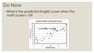
Example 1: Find the regression model for the given data. Compute the value of Y when X= 4. X Y 0 1 1 1.9 2 3.2 2.5 3.4 Dat asc
Solution: Apply the formula: Avg_x = 5.5/4 = 1.375 Avg_y = 9.5/4 = 2.375 X Y XY X^2 0 1 2 1 0 0 1 4 1.9 3.2 3.4 1.9 6.4 8.5 a1 = (16.8 4*1.375*2.375) / 11.25 4 * (1.375)^2 = 1.0136 2.5 Total: 6.25 5.5 9.5 16.8 11.25 a0 = 2.375 1.0136 * 1.375 = 0.9813 Hence, the required equation is Y = 0.9813 + 1.0136 X Prediction: When X=4, Y = 5.0357 Dat asc
Finding the best fit line: When working with linear regression, our main goal is to find the best fit line that means the error between predicted values and actual values should be minimized. The best fit line will have the least error. The different values for weights or the coefficient of lines (a0, a1) gives a different line of regression, so we need to calculate the best values for a0 and a1 to find the best fit line, so to calculate this we use cost function. Cost function: o The different values for weights or coefficient of lines (a0, a1) gives the different line of regression, and the cost function is used to estimate the values of the coefficient for the best fit line. o Cost function optimizes the regression coefficients or weights. It measures how a linear regression model is performing. o We can use the cost function to find the accuracy of the mapping function, which maps the input variable to the output variable. This mapping function is also known as Hypothesis function.
Finding the best fit line: For Linear Regression, we use the Mean Squared Error (MSE) cost function, which is the average of squared error occurred between the predicted values and actual values. It can be written as: Let s analyze what this equation actually means. yi = Actual output yi = predicted output Our goal is to minimize this mean, which will provide us with the best line that goes through all the points.
Finding the best fit line: Residuals: The distance between the actual value and predicted values is called residual. If the observed points are far from the regression line, then the residual will be high, and so cost function will high. If the scatter points are close to the regression line, then the residual will be small and hence the cost function. When we apply the regression equation on the given values of data, there will be difference between original values of y and the predicted values of y. Residual e = Observed value Predicted Value Sum of residuals = 0 = mean of residuals So, we try to find sum of squares of residuals, and then find its square root. This is known as Root Mean Squared Error (RMSE)
Finding the best fit line: Gradient Descent: o Gradient descent is used to minimize the MSE by calculating the gradient of the cost function. o A regression model uses gradient descent to update the coefficients of the line by reducing the cost function. o It is done by a random selection of values of coefficient and then iteratively update the values to reach the minimum cost function.
Multiple Linear Regressions In the previous topic, we have learned about Simple Linear Regression, where a single Independent/Predictor(X) variable is used to model the response variable (Y). But there may be various cases in which the response variable is affected by more than one predictor variable; for such cases, the Multiple Linear Regression algorithm is used. Moreover, Multiple Linear Regression is an extension of Simple Linear regression as it takes more than one predictor variable to predict the response variable. We can define it as: Multiple Linear Regression is one of the important regression algorithms which models the linear relationship between a single dependent continuous variable and more than one independent variable. Example: Prediction of CO2 emission based on engine size and number of cylinders in a car.
Multiple Linear Regressions Some key points about MLR: o For MLR, the dependent or target variable(Y) must be the continuous/real, but the predictor or independent variable may be of continuous or categorical form. o Each feature variable must model the linear relationship with the dependent variable. o MLR tries to fit a regression line through a multidimensional space of data-points. Assumptions for Multiple Linear Regression: o A linear relationship should exist between the Target and predictor variables. o The regression residuals must be normally distributed. o MLR assumes little or no multicollinearity (correlation between the independent variable) in data.
Multiple Linear Regressions More than one independent variables, X1, X2, and one dependent variable Y. Example: Predict temperature of the place based on humidity and pressure For two independent variables, given: (x1i, x2i , yi) for i= 1 . N Task is to find an equation that fits X1, X2 and Y The regression task is to predict yi+1 for a given value of x1i+1 and x2i+1
2 2 1 2 2 1 2 1 2 2 22 1 1 Dat asc