Graphical Solutions of Autonomous Equations in Mathematics II
Explore the graphical solutions of autonomous equations in Mathematics II taught by lecturer Wisam Hayder at Diyala University's College of Engineering. Learn about phase lines, equilibrium values, construction of graphical solutions, and sketching solution curves using phase lines. Dive into examples and understand the behavior of solution curves based on equilibrium values and concavity.

Download Presentation

Please find below an Image/Link to download the presentation.
The content on the website is provided AS IS for your information and personal use only. It may not be sold, licensed, or shared on other websites without obtaining consent from the author. Download presentation by click this link. If you encounter any issues during the download, it is possible that the publisher has removed the file from their server.
E N D
Presentation Transcript
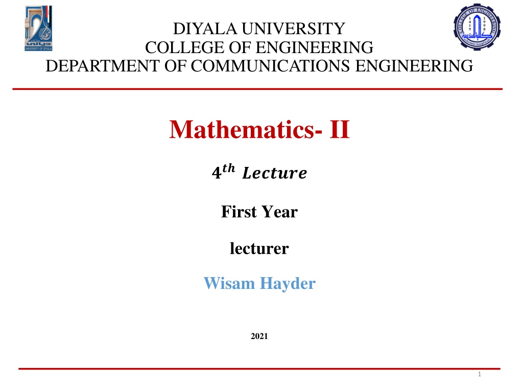
DIYALA UNIVERSITY COLLEGE OF ENGINEERING DEPARTMENT OF COMMUNICATIONS ENGINEERING Mathematics- II ?????????? First Year lecturer Wisam Hayder 2021 1
Graphical Solutions of Autonomous Equations The starting ideas for a graphical solution are the notions of phase line and equilibrium value. Equilibrium Values and Phase Lines 2
Graphical Solutions of Autonomous Equations Thus, equilibrium values are those at which no change occurs in the dependent variable, so y is at rest. The emphasis is on the value of y where dy /dx=0 , not the value of x, 3
Graphical Solutions of Autonomous Equations ??? ???????,the equilibrium values for the autonomous differential equation are y= -1 and y=2. To construct a graphical solution to an autonomous differential equation, we first make a phase line for the equation, a plot on the y-axis that shows the equation s equilibrium values along with the intervals where dy/ dx ?2? ??2are positive and negative. and 4
Graphical Solutions of Autonomous Equations Then we know where the solutions are increasing and decreasing,and the concavity of the solution curves. Example 1 Draw a phase line for the equation and use it to sketch solutions to the equation. 5
Graphical Solutions of Autonomous Equations FIGURE 9.15 Graphical solutions from Example 1 include the horizontal lines y = -1 and y = 2 through the equilibrium values. No two solution curves can ever cross or touch each other. 9
Graphical Solutions of Autonomous Equations Stable and Unstable Equilibria Look at Figure 9.15 once more, in particular at the behavior of the solution curves near the equilibrium values. Once a solution curve has a value near y = -1, it tends steadily toward that value; y = -1 is a stable equilibrium. 10
Graphical Solutions of Autonomous Equations The behavior near y =2 is just the opposite: all solutions except the equilibrium solution y = 2, itself move away from it as x increases. We call an unstable equilibrium. If the solution is at that value, it stays, but if it is off by any amount, no matter how small, it moves away. (Sometimes an equilibrium value is unstable because a solution moves away from it only on one side of the point.) 11
Graphical Solutions of Autonomous Equations Newton s Law of Cooling Modeling Newton s law of cooling. Here H is the temperature of an object at time t and ??is the constant temperature of the surrounding medium. Suppose that the surrounding medium (say a room in a house) has a constant Celsius temperature of 15 C. 12
Graphical Solutions of Autonomous Equations We can then express the difference in temperature as ?(?) 15. Assuming H is a differentiable function of time t, by Newton s law of cooling, there is a constant of proportionality k>0 such that (minus k to give a negative derivative when H > 15). 13
Graphical Solutions of Autonomous Equations Logistic Population Growth (5) model of exponential change for population growth Where k > 0 is the birth rate minus the death rate per individual per unit time. , maximum population M, growth rate k where r > 0 is a constant. Notice that k decreases as P increases toward M and that k is negative if P is greater than M. Substituting r(M- P) for k in Equation (5) gives the differential equation 18
Graphical Solutions of Autonomous Equations (6) The above model is referred to as logistic growth. 19
Systems of Equations and Phase Planes A Competitive-Hunter Model Imagine two species of fish, say trout and bass, competing for the same limited resources (such as food and oxygen) in a certain pond. We let x(t) represent the number of trout and y(t) the number of bass living in the pond at time t. In reality x(t) and y(t) are always integer valued, but we will approximate them with real-valued differentiable functions. This allows us to apply the methods of differential equations. 22
Systems of Equations and Phase Planes A large number of bass tends to cause a decrease in the number of trout, and vice-versa. Our model takes the size of this effect to be proportional to the frequency with which the two species interact, which in turn is proportional to xy , the product of the two populations. These considerations lead to the following model for the growth of the trout and bass in the pond: 23
Systems of Equations and Phase Planes Here x(t) represents the trout population, y(t) the bass population, and a, b, m, n are positive constants. A solution of this system then consists of a pair of functions x(t) and y(t) that gives the population of each fish species at time t. Each equation in (1) contains both of the unknown functions x and y, so we are unable to solve them individually. Instead, we will use a graphical analysis to study the solution trajectories of this competitive-hunter model. We now examine the nature of the phase plane in the trout-bass population model. 24
Systems of Equations and Phase Planes We will be interested in the 1st quadrant of the xy- plane, where x 0 and y 0 since populations cannot be negative. First, we determine where the bass and trout populations are both constant. Noting that the x(t) and y(t) values remain unchanged when ?? ?? = 0 and ?? ?? = 0 , Equations (1a and 1b) then become This pair of simultaneous equations has two solutions(x,y)=(0,0) and (x,y)= a b ). At these (x, y) values, called equilibrium or rest points, the two ( m n, populations remain at constant values over all time. 25
Ex 1. a. Identify the equilibrium values. Which are stable and which are unstable? b. Construct a phase line. Identify the signs of and c. Sketch several solution curves. 1.?? ??= (? + 2)(? 3) Sol. 31
?? ??= ?2 4 2. Sol. 33
Ex 2. The autonomous differential equations represent models for population growth. Use a phase line analysis to sketch solution curves for P(t), selecting different starting values P(0). Which equilibria are stable, and which are unstable? Sol. 34