Introduction to Motion Planning in Autonomous Robotics

Explore the concept of motion planning in autonomous robotics through graphical representations called roadmaps. Understand the importance of representation, transformations, and problem instances in motion planning algorithms. Learn about the accessibility and connectivity characteristics of roadmaps in constructing paths within free space regions.

Download Presentation

Please find below an Image/Link to download the presentation.
The content on the website is provided AS IS for your information and personal use only. It may not be sold, licensed, or shared on other websites without obtaining consent from the author. Download presentation by click this link. If you encounter any issues during the download, it is possible that the publisher has removed the file from their server.
E N D
Presentation Transcript
CS 485 Autonomous Robotics Motion Planning II Prof. Xuesu Xiao George Mason University Slides Credits: Gregory Stein 1
Logistics Start implementing motion controllers and planners in BARN. It s a good time to come up with a rough idea of your open-ended project. Assignment 1 due next week before class on Thursday Turn in paper copy or email the instructor and TA 2
Roadmaps What more can we do with state space search? Where do these graphs come from in practice? 3
We know how to search a graph: how can we relate that to motion planning? Roadmaps are graphical representations of the environment, and their relation to the physical world. ( or at least, toy examples that illustrate situations we will encounter in the real world.) Representation is important When studying combinatorial motion planning algorithms, it is important to carefully consider the definition of the input. What is the representation used for the robot and obstacles? What set of transformations may be applied to the robot? What is the dimension of the world? Are the robot and obstacles convex? Are they piecewise linear? The specification of possible inputs defines a set of problem instances on which the algorithm will operate. S. M. LaValle 4 From: S. M. LaValle: Planning Algorithms
We know how to search a graph: how can we relate that to motion planning? Roadmaps are graphical representations of the environment, and their relation to the physical world. ( or at least, toy examples that illustrate situations we will encounter in the real world.) A roadmap is a topological graph corresponding to some free space: Nodes in the graph, the set S, correspond to points in free space. From: S. M. LaValle: Planning Algorithms 5
An example region, from which we will construct a roadmap The space on the right defines our free space region. A roadmap has two defining characteristics: 1. Accessibility: that we can (easily) compute a path from any point in free space to a node in the graph. 2. Connectivity: that the graph can be used to define a path between any two of its nodes. From: S. M. LaValle: Planning Algorithms 6
An example region, from which we will construct a roadmap The space on the right defines our free space region. A roadmap has two defining characteristics: 1. Accessibility: that we can (easily) compute a path from any point in free space to a node in the graph. 2. Connectivity: that the graph can be used to define a path between any two of its nodes. So how do we make a roadmap? From: S. M. LaValle: Planning Algorithms 7
There are many ways to make a roadmap Many of these involve partitioning or decomposing the space. 8
A simple way of decomposing the space is the vertical cell decomposition also known as a Trapezoidal Decomposition 9
A simple way of decomposing the space is the vertical cell decomposition If you have polygonal obstacles, defined by some set of nodes and edges, computing this representation is done with a type of sweep algorithm. We travel from left-to-right and every time we encounter a node, we have to divide the space somehow: 10
A simple way of decomposing the space is the vertical cell decomposition This gives us some cells and the boundaries between them: 11
A simple way of decomposing the space is the vertical cell decomposition This gives us some cells and the boundaries between them. To get the roadmap, it is common to add points at the midpoint of all the vertical cell boundaries and at the center-of-mass for each trapezoid. Connectivity comes for free if you remember which cells are touching. 12
Vertical Cell Decomposition: is it a roadmap? There are two properties that define a roadmap: Does it satisfy Connectivity? 13
Vertical Cell Decomposition: is it a roadmap? There are two properties that define a roadmap: Does it satisfy Connectivity? Yes: can get between all nodes. 14
Vertical Cell Decomposition: is it a roadmap? There are two properties that define a roadmap: Does it satisfy Connectivity? Yes: can get between all nodes. Does it satisfy Accessibility? 15
Vertical Cell Decomposition: is it a roadmap? There are two properties that define a roadmap: Does it satisfy Connectivity? Yes: can get between all nodes. Does it satisfy Accessibility? Yes: can get from any point to a node 16
So are we done? No! Vertical Cell Decomposition yields suboptimal plans These paths could be made shorter by moving the edges closer to the obstacles. So we want a representation that allows us to get asymptotically close to the obstacles. 17
A visibility graph is a common way to build a roadmap in 2D polygonal environments If there are no obstacles, the shortest path between two points is a straight line. 18 From: CMU 15.381
A visibility graph is a common way to build a roadmap in 2D polygonal environments If there are no obstacles, the shortest path between two points is a straight line. But what if we add obstacles (polygonal ones for now)? 19 From: CMU 15.381
A visibility graph is a common way to build a roadmap in 2D polygonal environments If there are no obstacles, the shortest path between two points is a straight line. But what if we add obstacles (polygonal ones for now)? The shortest path seems to be a sequence of points joining object vertices. Is this always true? 20 From: CMU 15.381
A visibility graph is a common way to build a roadmap in 2D polygonal environments If there are no obstacles, the shortest path between two points is a straight line. But what if we add obstacles (polygonal ones for now)? The shortest path seems to be a sequence of points joining object vertices. Is this always true? Yes! (Proof by contradiction) 21 From: CMU 15.381
A visibility graph is a common way to build a roadmap in 2D polygonal environments The visibility graph involves computing which vertices can see which other vertices (and the start and goal points). Searching over this graph gives us the shortest path. 22 From: CMU 15.381
We can go even farther than visibility with the Shortest Path roadmap Notice that not all visibility edges are included. 23
Why dont we always use visibility graphs for planning? First: they get quite complicated and unwieldly in higher than 2 dimension. Also, we don t always want to be incredibly close to the obstacles. Sometimes it s better to be safer Other factors may play a role as well: it may be impossible for the robot (e.g., a self-driving car) to make sharp turns. Vehicle dynamics will play a big role for the next couple of weeks. 24
It is also common to create regular discrete grids out of otherwise continuous maps But turning a continuous space into a grid, you must trade off between a very small resolution (and high computational cost) or a big resolution (and miss closing off paths): This approach is therefore not complete in general! Image from: MIT 16.410 25
OctoMap (octrees) is a representation that allows for multi-resolution grid cells Key idea: if you need higher resolution, split a cell in half (in all dimensions). If not: keep a single big cell. Great for both large free space regions and small obstacles between them. https://octomap.github.io/ 26
OctoMap Server is great for fusing laser scan data into a grid https://www.youtube.com/watch?v=AodHUpuvJqs 27
Voronoi Diagrams: lets make a roadmap based on distance to obstacles Given a set of points in the plane, a Voronoi Diagram partitions space into regions based on proximity to the points: The line segments connecting these regions are equidistant to 2 points. The vertices are equidistant to 3. From: CMU 15.381 28
Voronoi Diagrams: lets make a roadmap based on distance to obstacles Given a set of points in the plane, a Voronoi Diagram partitions space into regions based on proximity to the points: The line segments connecting these regions are equidistant to 2 points. The vertices are equidistant to 3. From: CMU 15.381 29
Voronoi Diagrams: lets make a roadmap based on distance to obstacles From: CMU 15.381 30
Can we make Voronoi Diagrams from obstacles? Yes: the Generalized Voronoi Diagram Edges are piecewise, made up of straight lines and quadratic curves. Straight: equidistant from 2 edges Curved: equidistant from 1 corner and 1 edge 32
Can we make Voronoi Diagrams from obstacles? Yes: the Generalized Voronoi Diagram Edges are piecewise, made up of straight lines and quadratic curves. Straight: equidistant from 2 edges Curved: equidistant from 1 corner and 1 edge 33
Planning in a GVD works about as youd expect: Find a route to the nearest edge and then follow the edges to travel between the points (as computed by a search algorithm). Note: points on these lines are farthest from the nearest obstacles. This can be good for safety, but strongly depends on the problem. 34
Weaknesses of the Voronoi Diagram Like many of the other approaches we ve discussed, it s hard to compute them in higher dimensions. Also, they can be brittle/unstable: small changes in the environment can significantly change the GVD. Also, stay as far away from obstacles as you can isn t always the best planning objective. In most problem settings we don t need to be so conservative/cautious. 35
Summary of Roadmap Models Vertical Cell Decomposition Visibility Graph Generalized Voronoi Graph 36
Planning with movement costs Now we ll talk about how to plan over roadmaps: the edges have cost (often in units of time or distance) that need to be included when searching for the best path. In the coming weeks we ll talk about how to plan in environments where computing the graph is hard! What do we do when we cannot easily compute a roadmap? Planning with motion primitives Incorporating vehicle size, shape, and dynamics Sampling-based Planning 37
Add cost (path length) to the edges This means that our roadmap graph will include edge costs. These edge costs will also be added to our search tree and incorporated into the total path cost at each node. 0 2 3 4 2 2 2 6 1 5 5 8 38
Finding the shortest path: a problem statement The input to our search problem now includes a weight function: where (a function that outputs a cost for pairs of vertices) The output is now a simple path from S to G that (ideally) has the shortest path weight (and optionally also returns the weight of the path). 39
Whats the simplest way to find the shortest path we can think of? 40
Whats the simplest way to find the shortest path we can think of? How about we just grow outward from the starting node in order of cost: Uniform Cost Search 41
Whats the simplest way to find the shortest path we can think of? How about we just grow outward from the starting node in order of cost: Uniform Cost Search Similar to breadth-first search, except instead of using the steps in the path to order Q, we use path cost of to order Q. Grows outward from the start until the goal is reached. Visually: 42
Uniform-Cost Search: An Example 43 From: MIT 16.410
Uniform-Cost Search: An Example 44 From: MIT 16.410
Uniform-Cost Search: An Example 45 From: MIT 16.410
Uniform-Cost Search: An Example 46 From: MIT 16.410
Uniform-Cost Search: An Example We reached the goal! are we done? 47 From: MIT 16.410
Uniform-Cost Search: An Example We reached the goal! are we done? Maybe not, so let s keep going. 48 From: MIT 16.410
Uniform-Cost Search: An Example We reached the goal! are we done? Maybe not, so let s keep going. Look: we found a new path to the goal that s shorter! 49 From: MIT 16.410
Uniform-Cost Search: An Example We reached the goal! are we done? Maybe not, so let s keep going. Look: we found a new path to the goal that s shorter! 50 From: MIT 16.410


 is a representation that")


 to the edges")