Low Frequencies for Inversion of Reflections
"Exploring the use of low frequencies for inversion of reflections in seismic data processing. The presentation covers motivations for tau-p inversion, direct and indirect methods, and discusses the transformation of hyperbolic reflections into ellipses. Various inversion techniques, applications in unconventional resources, gas hydrates, and more are also outlined."

Download Presentation

Please find below an Image/Link to download the presentation.
The content on the website is provided AS IS for your information and personal use only. It may not be sold, licensed, or shared on other websites without obtaining consent from the author. Download presentation by click this link. If you encounter any issues during the download, it is possible that the publisher has removed the file from their server.
E N D
Presentation Transcript
Low Frequencies for Inversion of Reflections Lasse Amundsen, rjan Pedersen and Rune Mittet
Outline Motivation for tau-p inversion Indirect tau-p inversion: FWI with Gauss-Newton scheme Direct tau-p inversion: Scaling ( AVA ) and stretching ( residial migration ) the gradient of constant velocity inversion ( c-v migration ) Discussion/Conclusion Hyperbolic reflections transform into ellipses, straight events into points. ?(?) Phase velocity ?(?,?) = 1 ??(?)2
Motivation for tau-p reflection inversion Amundsen and Ursin 1991 F-K inversion of acoustic data: Geophysics 56 1027-1039 Fast, elastic Newton-type inversions for VP, VS, density, attenuation Zhao, Ursin and Amundsen 1994 F-K elastic inversion: Geophysics 59 1868-1881 Used where geology is flattish Amundsen, Reitan and Arntsen 2005 Geometric analysis of data-driven inversion/depth imaging: JSE 14 51-62 Amundsen, Reitan, Helgesen and Arntsen 2005 Data-driven inversion/depth imaging: Inverse Problems 21 1823-50 1. Unconventionals: sweet spot mapping 2. Gas hydrates 3. Temperature changes of water column 4. Starting model for general FWI Amundsen, Reitan, Arntsen and Ursin 2006 Acoustic AVA inversion/depth imaging: Inverse Problems 22 1921-45 Amundsen, Reitan, Arntsen and Ursin 2008 Elastic AVA inversion/depth imaging: Inverse Problems 22 1921-45 Understand the potential, pitfalls, and limitations of FWI 1. What can the gradient (of the misfit function) offer you today ? 2. Effect of missing low frequencies Assumtions in this presentation 1. Acoustic wave equation; constant density 2. Known wavelet
? ? =1 ? (?) ?(?) 2 Misfit function is sum over frequencies ? ? = ?? ? Gradient of misfit function ? = ?2? ? Hessian ? = ? 1? Model update I. FWI with Gauss-Newton method In tau-p, the gradient can be found analytically when - the sum over frequencies ranges from to + infinity - the wavelet is unity Essentially, the gradient becomes a sum of step functions which is great since it contains information about the velocity profile. The high frequencies are not important. Take out low frequencies, and the gradient will change.
Slab velocity model and tau-data for p=0 ?1 Model parameters M=100 # frequencies N=120 (up to 30 Hz)
Gradient and velocity updates (GN inversion) ?1 Start model: Constant velocity Iterations 1,2,3 and 10 1 2 3 1 2 3 The gradients have layer or box- structure.
Hessian and its inverse (iteration 10) Since the gradients have layer-structure, the inverse Hessians do not need to do a big job. No stabilization is needed.
Gradients without and with low frequencies 1 23 2 3 fmin<1.25 Hz fmin=1.25 Hz 1 What can the gradient (of the misfit function) offer you today ?
Velocity inversion without and with low frequencies fmin<1.25 Hz fmin=1.25 Hz Both models produce exactly the same data and reduce misfit by 10 6
II. Scaling and streching the gradient from constant-velocity inversion ?(?) Scaling g to get phase velocity v but in squeezed geometry; Scaling = AVA ? ?,? = ?[?1, ?,? ?,? ] ; ? ?,? = 1 1 ??(?)2 ? ?? ? ?,? ?1(?) Stretching v to phase velocity in correct geomery; Stretching = Residual migration ? ?,? = ? ?, 2 0 c1, v1 is water-speed velocity note that scale and stretch depend only on gradient s amplitude!
Velocity model and data (p=0 and p=0.75/c1) p=0 p=0.75/c1
Constant-velocity gradients in pseudo-depth ? ? = 0,? ?(0) ?? ? ? =0.75 ?1 ?(?) ,? ?1 2 Apply AVA to gradient ? : ? ?,? = ?[?1, ?,? ?,? ] ????: ??=1 ?(0) ?(?) 2) 1 (1 ??1 ?
Scale gradients to phase velocity ? ? = 0,? ?1(? = 0) ? ? =0.75 ,? ?1 Apply residual migration to ?: ? ?? ? ?,? ?1(?) ?1(?) ? ?,? = ? ?, 0
Residual migration (stretching) p=0 p=0.75/c1 Residual migration to ?: ? ?? ? ?,? ?1(?) ? ?,? = ? ?, 0
Discussion/Conclusion Need low frequencies to calculate a gradient that carries information of layer velocities The Hessian can partly correct the gradient for missing low frequencies Scaling and stretching the gradient shown for plane-layer tau-p inversion need generalization to laterally varying medium tougher problem to handle


")
")


")