Multivariate Adaptive Regression Splines (MARS) in Machine Learning

Slide Note

Multivariate Adaptive Regression Splines (MARS) offer a flexible approach in machine learning by combining features of linear regression, non-linear regression, and basis expansions. Unlike traditional models, MARS makes no assumptions about the underlying functional relationship, leading to improved interpretability and performance. By using a piecewise linear basis expansion approach, MARS allows for local operations, resulting in a more parsimonious regression surface. This adaptive nonparametric regression procedure is ideal for capturing complex relationships in high-dimensional spaces.

pgent Follow

Uploaded on Oct 09, 2024 | 0 Views

Download Presentation

Please find below an Image/Link to download the presentation.

The content on the website is provided AS IS for your information and personal use only. It may not be sold, licensed, or shared on other websites without obtaining consent from the author. Download presentation by click this link. If you encounter any issues during the download, it is possible that the publisher has removed the file from their server.

E N D

Presentation Transcript

Multivariate Adaptive Regression Splines (MARS) BMTRY 790: Machine Learning

Decision Trees: Concerns We recently discussed tree-based methods Non-parametric and semi-parametric methods Models can be represented graphically for easy interpretation Intuitive and easy to interpret relative to many statistical models Similar to how clinicians think to make decisions about patient care There are issues however with decision tree methods: Have a tendency to over-fit the data (not uncommon among machine learning methods) Referred to as weak learners Small changes in the data results in very different models

Multivariate Adaptive Regression Splines (MARS) Linear regression, linear basis expansions, and non-linear regression all make assumptions about the model Incorrect assumptions lead to poor results Reduced interpretability CART (and similar) models interpretable but have the issues discussed previously Also tend to perform poorly for regression tasks (i.e. continuous outcomes) Difficulty capturing additive relationships Can we combine several features of these approaches? Basis functions Minimal a priori assumptions Reasonable computational complexity "good" error rates

Multivariate Adaptive Regression Splines (MARS) Adaptive nonparametric regression procedure Makes no assumption about any underlying functional relationship Constructs models from a set of coefficients and basis functions that are entirely "driven" by the data Partition feature space into regions, each with its own regression equation Recall we used this idea in CART Also makes it useful for larger number of inputs (high dimension)

Multivariate Adaptive Regression Splines (MARS) MARS uses a piecewise linear basis expansion approach x t x t t x x t if if ( ) ( ) x t = = t x and + + 0 0 otherwise otherwise

Advantages of MARS Approach Key advantage to MARS is that features are allowed to operate locally Only regions where inputs or cross-products are non-zero impact prediction Result: regression surface that is built in a parsimonious manner Also has a computational advantage by using piecewise linear basis expansions Exploits form of basis function when evaluating choice of knots Needs only O(N) operations Forward modeling strategy means higher-order interactions only considered when the lower-order versions are in the model Thus avoid searching over exponentially growing space of possible models

More on MARS Each function estimated for a MARS model is piecewise linear with a knot at t i.e. these are linear splines Idea: Generate reflected pairs for each feature Xjwith knots at unique xijyielding a collection of basis functions (recall the figure) ( ) ( + ) = = , 1,2,..., C X t t X j N j j + , ,..., t x x x 1 2 j j Nj If all values in X are unique, there will be 2Np basis functions Each basis function depends only on a single Xj

Building a MARS Model Use a forward stepwise approach using functions from set C and their products to yield a model + ( ) f X ( ) X M = h 0 m m = 1 m For the selected hm(X), coefficients mestimated using OLS approach i.e. estimate based on minimizing residual sums of squares So how do we determine what basis functions are added to the model as the algorithm progresses

Building a MARS Model Start with the constant model with hm(X) = 1 Consider all functions in C as candidate functions At each stage, consider Reflected pairs in C Products of functions hm(X) in current model set M with reflected pairs in C In general considered for inclusion: ( ) X = = 1 h 0 ( ) ( ( ) ( X ) ) ( ) X = h h X X x 1 m j ij + = h x X 2 ij j +

Results is a 3-D Surface

Building a MARS Model At each step, the reflected pair and product with hm(X) that yield the largest decrease in training error added to the model The terms added to the model take the form ( ) ( h X ) ( ) ( h X ) + M , X t t X h + + 1 2 M l j M l j l + + MARS can consider higher order interactions (i.e. multiply more than 2 linear basis functions) but interpretability can be tough One restriction placed on model terms is that each input can only appear in a product once

Example The algorithm might proceed as follows

Overfitting and MARS Large number of basis functions/interactions makes it easy to over fit MARS uses GCV to determine the appropriate number of model parameters ( ( ) ( 1 M ) 2 ( ) x f N y ( ) ( ) i i = 1 i = = + GCV M r cK where ) 2 N r = number of independent basis functions K = number of knots c = constant 2 if model includes only additive terms 3 if model includes products

Overfitting and MARS Most implementations of MARS still fit to a full model using a forward step-wise approach As terms added to the model, both sides of the reflected pair are included ( ) ( ) + + k X x x X Step add: 1 k j ij k ij j + + Once the full model is constructed, pruning implemented via backward step-wise selection The GCV used to conduct the backward selection Under pruning Not required to include both sides of the reflected pair Also not required to include main effects when interactions are present

Comparison of MARS and CART Note: MARS and CART are strongly related to one another Following modification to MARS yields the same results as CART Replace the piecewise linear basis functions in MARS with step functions ( ) ( ) 0 0 I x t I t x and Model terms multiplied by a candidate term are replaced by the interaction and thus not available for additional interactions However, implementation of MARS allows the models to capture additive effects that one can t identify directly with CART

Fitting a MARS Model in R There are (at least) 2 R libraries that can be used to fit MARS models mda: Developed by Hastie and Tibshirani Uses GCV approach to select model and can prune models as well Also has functions to fit models by several related methods earth (Enhanced Adaptive Regression Through Hinges) Specifically for fitting MARS models More functionality than mda Has a function to convert MARS models fit in mda to an earth object

Example: Immune Response Recall our environmental exposure and immune response data Endocrine Disrupting Compounds (EDCs) are ubiquitous natural and man- made chemicals found in consumer products that have the ability to mimic natural hormones. Studies suggest EDCs may induce an inflammatory response. Study goal to evaluate impact of environmental EDC levels on inflammatory Study population 75 serum samples Predictors: levels of 9 EDCs Outcome: Level of inflammatory cytokine INF

mda Package ### Fitting MARS model using mda pakage library(mda) immresp<-read.csv("H:\\public_html\\BMTRY790_Spring2023\\Datasets\\EnvironContamImmuneResp2.csv") ### Fitting an ADDITIVE MARS model using the mda package mars.fit1<-mars(immresp[,-10], immresp[,10], degree=1, prune=TRUE, forward.step = TRUE) names(mars.fit1) [1] "call" "all.terms" "selected.terms" "penalty" "degree" "nk" [7] "thresh" "gcv" "factor" "cuts" "residuals" "fitted.values" [13] "lenb" "coefficients" "x"

mda Package ### Information about our ADDITIVE MARS model mars.fit1$gcv [1] 371.9659 mars.fit1$all.terms [1] 1 2 3 4 5 6 7 8 10 11 12 13 14 15 16 17 18 20 21 mars.fit1$selected.terms [1] 1 3 5 8 mars.fit1$coef [,1] [1,] 23.4345 [2,] 0.0578 [3,] 330.817 [4,] 0.0451

mda Package mars.fit1$cuts [,1] [,2] [,3] [,4] [,5] [,6] [,7] [,8] [,9] [1,] 0.0 0 0.0 0 0.00 0.00 0.00 0.00 0 [2,] 0.0 0 0.0 0 0.00 0.00 0.00 0.00 919 [3,] 0.0 0 0.0 0 0.00 0.00 0.00 0.00 919 [4,] 0.1 0 0.0 0 0.00 0.00 0.00 0.00 0 [5,] 0.1 0 0.0 0 0.00 0.00 0.00 0.00 0 [6,] 0.0 0 0.0 21 0.00 0.00 0.00 0.00 0 [7,] 0.0 0 0.0 21 0.00 0.00 0.00 0.00 0 [8,] 0.0 0 0.0 0 0.00 0.00 0.00 0.00 580 [9,] 0.0 0 0.0 0 0.00 0.00 0.00 0.00 580 [10,] 0.0 0 0.0 0 0.00 4.66 0.00 0.00 0 [11,] 0.0 0 0.0 0 0.00 4.66 0.00 0.00 0 [12,] 0.0 0 0.0 0 0.00 0.00 9.43 0.00 0 [13,] 0.0 0 0.0 0 0.00 0.00 9.43 0.00 0 [14,] 0.0 0 0.0 0 0.00 0.00 0.00 32.46 0 [15,] 0.0 0 0.0 0 0.00 0.00 0.00 32.46 0 [16,] 0.0 0 0.0 0 8.36 0.00 0.00 0.00 0 [17,] 0.0 0 0.0 0 8.36 0.00 0.00 0.00 0 [18,] 0.0 0 0.0 0 12.3 0.00 0.00 0.00 0 [19,] 0.0 0 0.0 0 12.3 0.00 0.00 0.00 0 [20,] 0.0 0 28.9 0 0.00 0.00 0.00 0.00 0 [21,] 0.0 0 28.9 0 0.00 0.00 0.00 0.00 0

mda Package mars.fit1$factor PFHxA PFHpA PFOA PFUnA PFDoA PFTriA PFHxS PFHpS PFOS [1,] 0 0 0 0 0 0 0 0 0 [2,] 0 0 0 0 0 0 0 0 1 [3,] 0 0 0 0 0 0 0 0 -1 [4,] 1 0 0 0 0 0 0 0 0 [5,] -1 0 0 0 0 0 0 0 0 [6,] 0 0 0 1 0 0 0 0 0 [7,] 0 0 0 -1 0 0 0 0 0 [8,] 0 0 0 0 0 0 0 0 1 [9,] 0 0 0 0 0 0 0 0 -1 [10,] 0 0 0 0 0 1 0 0 0 [11,] 0 0 0 0 0 -1 0 0 0 [12,] 0 0 0 0 0 0 1 0 0 [13,] 0 0 0 0 0 0 -1 0 0 [14,] 0 0 0 0 0 0 0 1 0 [15,] 0 0 0 0 0 0 0 -1 0 [16,] 0 0 0 0 1 0 0 0 0 [17,] 0 0 0 0 -1 0 0 0 0 [18,] 0 0 0 0 1 0 0 0 0 [19,] 0 0 0 0 -1 0 0 0 0 [20,] 0 0 1 0 0 0 0 0 0 [21,] 0 0 -1 0 0 0 0 0 0

MARS Model from mda ### So using this info we can get the form of our MARS model mars.fit1$coef [1,] 23.4345 [2,] 0.0578 [3,] 330.817 [4,] 0.0451 mars.fit1$cuts[c(1,3,5,8),] [,1] [,2] [,3] [,4] [,5] [,6] [,7] [,8] [,9] [1,] 0.0 0 0.0 0 0.00 0.00 0.00 0.00 0 [3,] 0.0 0 0.0 0 0.00 0.00 0.00 0.00 919 [5,] 0.1 0 0.0 0 0.00 0.00 0.00 0.00 0 [8,] 0.0 0 0.0 0 0.00 0.00 0.00 0.00 580 mars.fit1$factor[c(1,3,5,8),] PFHxA PFHpA PFOA PFUnA PFDoA PFTriA PFHxS PFHpS PFOS [1,] 0 0 0 0 0 0 0 0 0 [3,] 0 0 0 0 0 0 0 0 -1 [5,] -1 0 0 0 0 0 0 0 0 [8,] 0 0 0 0 0 0 0 0 1

What Is The Actual Model? = ( ) x ( ) x f 3 = y h m m = 0 m

Example Predictions What is our prediction for PFOS = 975 and PFHxA = 0.05?

Example Predictions What about for PFOS = 375 and PFHxA = 0.26? And for PFOS = 680 and PFHxA = 0.04?

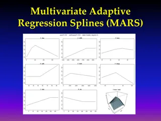
Effects of Each Predictor ### PLOTTING ALL INDIVIDUAL PREDICTORS par(mfrow = c(3, 3), mar=c(4,3,3,2), pty="s") for (i in 1:9) { xp <- matrix(sapply(immresp[,-10], mean), nrow(immresp), ncol(immresp) - 1, byrow = TRUE) xr <- sapply(immresp, range) xp[, i] <- seq(xr[1, i], xr[2, i], len=nrow(immresp)) xf <- predict(mars.fit1, xp) plot(xp[, i], xf, xlab = colnames(immresp)[i], ylab = "", type = "l") }

Response Surface

Interactions in MARS ### Fitting an INTERACTION MARS model using the mda package mars.fit2<-mars(immresp[,-c(2:6,9)], immresp[,10], degree=2, prune=TRUE, forward.step = TRUE) mars.fit2$gcv [1] 425.879 mars.fit2$all.terms [1] 1 2 3 4 5 6 8 9 10 12 13 14 15 16 18 20 21 mars.fit2$selected.terms [1] 1 2 5 mars.fit2$coef [,1] [1,] 47.6428 [2,] 0.0341 [3,] 0.0123

Interactions in MARS ### So using this info we can get the form of our MARS model mars.fit2$coef [1,] 47.6428 [2,] 0.0341 [3,] 0.0123 mars.fit2$cuts[c(1,2,5),] [,1] [,2] [,3] [,4] [,5] [,6] [1,] 0 0 0.0 0 0 0 [2,] 0 0 0.0 0 0 919 [3,] 0 0 19.5 0 0 919 mars.fit2$factor[c(1,2,5),] PFHpA PFOA PFUnA PFDoA PFTriA PFOS [1,] 0 0 0 0 0 0 [2,] 0 0 0 0 0 1 [3,] 0 0 -1 0 0 -1

What Is the Model Allowing for Interactions? = ( ) x ( ) x f 2 = y h m m = 0 m

Example Predictions (Interaction Model) What is our prediction for PFOS = 180 and PFUnA = 14.2? Is there a region where both model terms have an impact?

Effects of Each Predictor par(mfrow = c(2, 3), mar=c(4,3,3,2), pty="s") for (i in 1:6) { xp <- matrix(sapply(immresp[,c(2:6,9)], mean), nrow(immresp), 6, byrow = TRUE) xr <- sapply(immresp[,c(2:6,9)], range) xp[, i] <- seq(xr[1, i], xr[2, i], len=nrow(immresp)) xf <- predict(mars.fit2, xp) plot(xp[, i], xf, xlab = colnames(immresp) [c(2:6,9)][i], ylab = "", type = "l") }

Response Surface (Interaction Model)

earth Package ### Fitting an ADDITIVE MARS model using the earth package mars.fit3<-earth(immresp[,-10], immresp[,10], degree=1, prune=TRUE, forward.step = TRUE) mars.fit3 Selected 9 of 16 terms, and 4 of 9 predictors Termination condition: Reached nk 21 Importance: PFOS, PFHxA, PFUnA, PFTriA, PFHpA-unused, PFOA-unused, PFDoA-unused, PFHxS-unused, PFHpS-unused Number of terms at each degree of interaction: 1 8 (additive model) GCV 376.3404 RSS 16880.12 GRSq 0.2197695 RSq 0.5206911 names(mars.fit3) [1] "rss" "rsq" "gcv" "grsq" "bx" [6] "dirs" "cuts" "selected.terms" "prune.terms" "fitted.values" [11] "residuals" "coefficients" "rss.per.response" "rsq.per.response" "gcv.per.response" [16] "grsq.per.response" "rss.per.subset" "gcv.per.subset" "leverages" "pmethod" [21] "nprune" "penalty" "nk" "thresh" "termcond" [26] "weights" "call" "namesx.org" "namesx"

earth Package ### Fitting an ADDITIVE MARS model using the earth package mars.fit3$coef immresp[,10] (Intercept) 40.26172178 h(914-PFOS) 0.03890829 h(PFHxA-0.13) 370.02511425 h(20.8-PFUnA) 4.60377589 h(PFOS-594) 0.03927793 h(PFTriA-3.76) -224.01447772 h(PFTriA-4.08) 122.52065846 h(PFTriA-3.38) 103.71368915 h(PFHxA-0.07) -367.77967552

earth Package mars.fit3$selected.terms [1] 1 3 4 7 8 9 14 15 16 mars.fit3$cuts PFHxA (Intercept) 0.00 0 0 h(PFOS-914) 0.00 0 0 h(914-PFOS) 0.00 0 0 h(PFHxA-0.13) 0.13 0 0 h(0.13-PFHxA) 0.13 0 0 h(PFUnA-20.8) 0.00 0 0 h(20.8-PFUnA) 0.00 0 0 h(PFOS-594) 0.00 0 0 h(PFTriA-3.76) 0.00 0 0 h(3.76-PFTriA) 0.00 0 0 h(PFHxS-9.87) 0.00 0 0 h(9.87-PFHxS) 0.00 0 0 h(PFHxS-34.02) 0.00 0 0 h(PFTriA-4.08) 0.00 0 0 h(PFTriA-3.38) 0.00 0 0 h(PFHxA-0.07) 0.07 0 0 PFHpA PFOA PFUnA PFDoA PFTriA 0.0 0 0.0 0 0.0 0 0.0 0 0.0 0 20.8 0 20.8 0 0.0 0 0.0 0 0.0 0 0.0 0 0.0 0 0.0 0 0.0 0 0.0 0 0.0 0 PFHxS 0.00 0 0.00 0 0.00 0 0.00 0 0.00 0 0.00 0 0.00 0 0.00 0 0.00 0 0.00 0 9.87 0 9.87 0 34.02 0 0.00 0 0.00 0 0.00 0 PFHpS PFOS 0.00 0.00 0.00 0.00 0.00 0.00 0.00 0.00 3.76 3.76 0.00 0.00 0.00 4.08 3.38 0.00 0 914 914 0 0 0 0 594 0 0 0 0 0 0 0 0

earth Package mars.fit3$dirs.[mars.fit3$selected.terms,] PFHxA PFHpA PFOA PFUnA PFDoA PFTriA PFHxS PFHpS PFOS (Intercept) 0 0 0 0 0 0 0 0 0 h(914-PFOS) 0 0 0 0 0 0 0 0 -1 h(PFHxA-0.13) 1 0 0 0 0 0 0 0 0 h(20.8-PFUnA) 0 0 0 -1 0 0 0 0 0 h(PFOS-594) 0 0 0 0 0 0 0 0 1 h(PFTriA-3.76) 0 0 0 0 0 1 0 0 0 h(PFTriA-4.08) 0 0 0 0 0 1 0 0 0 h(PFTriA-3.38) 0 0 0 0 0 1 0 0 0 h(PFHxA-0.07) 1 0 0 0 0 0 0 0 0

Diagnostic Plots for earth plot(mars.fit3) Note, the GRSq is: GCV GCV 1 null

Converting a MARS from mda to earth ### We can convert a MARS model developed in mda into the format observed in earth using the earth package mars.fit4<-mars.to.earth(mars.fit2) mars.fit4 Selected 3 of 18 terms, and 2 of 6 predictors Termination condition: Unknown Importance: object has no prune.terms, call update() on the model to fix that Number of terms at each degree of interaction: 1 1 1 GCV 425.879 RSS 27034.8 GRSq 0.1170658 RSq 0.2323503 update(mars.fit4) Termination condition: Unknown Importance: PFOS, PFUnA, PFHpA-unused, PFOA-unused, PFDoA-unused, PFTriA-unused Number of terms at each degree of interaction: 1 1 1 GCV 425.879 RSS 27034.8 GRSq 0.1170658 RSq 0.2323503

Diagnostic Plots for MARS from mda using earth plot(mars.fit4)

Recall Our Concerns with Decision Trees Single decision trees methods have a tendency to over-fit the data They also tend to be rather weak classifiers Small changes in the training data can result in very different models Test error rate may be only slightly better than guessing MARS was designed to address poor regression performance of an approach like CART Can still have issues with over-fitting and poor test performance This leads us to a discussion of methods to improve the performance of these models!