Understanding Probabilistic Graphical Models in Real-world Applications
Probabilistic Graphical Models (PGMs) offer a powerful framework for modeling real-world uncertainties and complexities using probability distributions. By incorporating graph theory and probability theory, PGMs allow flexible representation of large sets of random variables with intricate relationships. Challenges such as model size and variable independence are addressed through structured graph representations, providing a robust foundation for solving problems with probabilistic uncertainty.

Download Presentation

Please find below an Image/Link to download the presentation.
The content on the website is provided AS IS for your information and personal use only. It may not be sold, licensed, or shared on other websites without obtaining consent from the author. Download presentation by click this link. If you encounter any issues during the download, it is possible that the publisher has removed the file from their server.
E N D
Presentation Transcript
Probabilistic Graphical Models Part 1: Overview and Applications
Outline Motivation for Probabilistic Graphical Models Applications of Probabilistic Graphical Models Graphical Model Representation
Probabilistic Modeling1 when trying to solve a real-world problem using mathematics, it is common to define a mathematical model of the world, e.g. Y = ?? often, the real world that we are trying to model involves a significant amount of uncertainty (e.g., the price of a house has a certain chance of going up if a new subway station opens within a certain distance). to deal with uncertainty we usually model the world in the form of a probability distribution P(X, Y) X, Y are random variables
Challenges of Probabilistic Modeling1 Assume a (probabilistic) model P (Y, X1, X2, Xn) of word occurrences in spam and non-spam mail: Each binary variable Xi encodes whether the ith English word is present in the email The binary variable Y indicates whether the email is spam In order to classify a new email, we look at the probability P(Y = 1| X1, X2, Xn)
Challenges and Opportunities of Probabilistic Modeling1 Assume a (probabilistic) model P (Y, X1, X2, Xn) of word occurrences in spam and non-spam mail: The size (domain) of P is huge (2N+1, N being the size of the English vocabulary) Independence among variables can significantly decrease that domain: However: the conditional independence assumption among all the variables does not always result in a good prediction model (e.g., pharmacy and pills are probably highly dependent) Nonetheless: some variables are independent of each other (e.g., muffin and penguin )
Challenges and Opportunities of Probabilistic Modeling1 Statistical independence conditions can be described and represented with a graph structure: P(X1, X2, , Xn | y) = P(X1|y) * P(X2|y) * *P(Xn|y)
Probabilistic Modeling1 Probabilistic Graphical Models(PGMs) form a powerful framework for representing/modeling complex real world domains using probability distributions. They: bring together graph theory and probability theory provide a flexible framework for modeling large collections of random variables with complex interactions enable the explicit representation of independences between variables with graphs leverage the graph representation to discover efficient (exact or approximate) inference and learning algorithms form the basis of causality theory
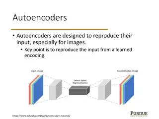
Applications1 Image processing unsupervised feature generation3,10 in-painting (reconstruction of small damaged portion of images)8 image denoising9 Audio speech synthesis7 speech recognition6 Information/Coding Theory:error-correcting codes Computer Science:spam filtering/document classification (Bayesian models have been used in the Gmail spam filtering algorithm) Computer Networks cooperative localization time scheduling
Applications1 Science Computational Biology5:computational network biology Genetics:Bayesian Networks are used in Gene Regulatory Networks to model cell behavior and to form relevant predictions Ecology: used to study phenomena that evolve over space and time, capturing spatial and temporal dependencies (e.g., bird migrations) Economics : can model spatial distributions of quantities of interests (e.g., assets or expenditures-based measures of wealth) Healthcare and Medicine Disease Diagnosis4: used to model the possible symptoms and predict whether a person is infected/diseased etc. Biomonitoring: Bayesian Networks play an important role in monitoring the quantity of chemical dozes used in pharmaceutical drugs Transportation:traffic analysis
Graphical Model Representation1 In PGMs the relationships between random variables are described by graphs whose properties (e.g., connectivity, tree-width) reveal probabilistic and algorithmic features of the model (e.g., independence, learning complexity). Directed Graphical Models (DGMs) : employ directed graphs directed edges describe causality relationship between random variables Undirected Graphical Models (UGMs) : employ undirected graphs Moralized Graphs: undirected versions of DGMs Conditional Random Fields: discriminative incarnation of UGMs Factor Graphs: both variables and functions are represented in the graph Latent Variable Models: DGMs or UGMs where some variables are never observed Models with Continuous Variables
Directed Graphical Models1 A Directed Graphical Model (Bayesian Network) is a directed graph G = (V, E) together with: a random variable Xi associated with each node i V a conditional probability distribution P(Xi XAi) for each Xi, specifying the probability of Xiconditioned on its parents values That Bayesian network defines the probability distribution ??(Xi XAi). We say that a probability factorizes over a DAG G if it can be decomposed into a product of factors, as specified by G.
Directed Graphical Models2 Bayesian network model for lung cancer diagnosis: p(is_smoking = T) = 0.2 p(is_smoking = F) = 0.8 is_smoking has_lung_cancer has_bronchitis p(has_lung_cancer = T | is_smoking = T) = 0.3 p(has_lung_cancer = F | is_smoking = T) = 0.7 p(has_bronchitis = T | is_smoking = T) = 0.25 p(has_bronchitis = F | is_smoking = T) = 0.75 p(has_lung_cancer = T | is_smoking = F) = 0.005 p(has_lung_cancer = F | is_smoking = F) = 0.995 p(has_bronchitis = T | is_smoking = F) = 0.05 p(has_bronchitis = F | is_smoking = F) = 0.95 has_abnormal_X-rays p(has_abnormal_X-rays = T | has_lung_cancer = T) = 0.6 p(has_abnormal_X-rays = F | has_lung_cancer = T) = 0.4 p(has_abnormal_X-rays = T | has_lung_cancer = F) = 0.02 p(has_abnormal_X-rays = F | has_lung_cancer = F) = 0.98
Directed Graphical Models2 Bayesian network model for lung cancer diagnosis. It defines the joint probability distribution: P(has_abnormal_X-rays, has_lung_cancer, has_bronchitis, is_smoking) = P(is_smoking) * P(has_lung_cancer | is_smoking) * P(has_bronchitis | is_smoking) * P(has_abnormal_X-rays | has_lung_cancer)
Directed Graphical Models2 Bayesian network model for lung cancer diagnosis. It defines the probability distribution: P(has_abnormal_X-rays, has_lung_cancer, has_bronchitis, is_smoking) = P(is_smoking) * P(has_lung_cancer | is_smoking) * P(has_bronchitis | is_smoking) * P(has_abnormal_X-rays | has_lung_cancer) This distribution can be represented with 7 parameters as opposed to 24- 1 = 15 parameters that the distribution with no independence assumptions needs
Relationships described by Directed Graphical Models2 Independencies can be recovered from a DGM graph by looking at three types of structures: Cascade (a), (b): if Z is observed X Y | Z Common Parent (c) : if Z is observed X Y | Z V-structure (d) if Z is unobserved X Y | Z The above rules are applied recursively on larger graphs
Undirected Graphical Models1 An Undirected Graphical Model or Markov Random Field (MRF) is a probability distribution P over variables X1, X2, ,Xn defined by an undirected graph G in which: each node i correspond to a variables Xi the probability P has the form 1 ? ? ? (??) ? ?1,?2, ,?? = negative function (usually called potential function) over all the variables in a clique. where C denotes the set of cliques (i.e., fully connected subgraphs) of G, and each c is a non- the partition function: ? = ?,?2, ,?? ? ? (??) is a normalization constant to ensure that the distribution sums up to 1 the potential functions simply define related variables and quantify the strength of their interactions
Undirected Graphical Models2 An MRF to model voting preferences among four people: Alice (A), Bob (B), Charlie (C), David (D). Assume an election against two (2) candidates. Also assume (A, B), (B, C), (C, D) and (D, A) are friends. Friends tend to have similar voting preferences: Alicevote Bobvote Davidvote Charlievote
Undirected Graphical Models2 One way to define a probability over the joint voting decision of A, B, C, D is to assign scores to each assignment of these variables and then define a probability as the normalized score. We define the score as: ?(?,?,?,?) = ?,? ?,? * ?,? * ?,? where (X, Y) is defined as: X Y 1 1 10 0 0 5 1 0 1 0 1 1 then: 1 ? * ? ?,?,?,? , ? = ?,?,?,? ? ?,?,?,? ? ?,?,?,? =
Undirected Graphical Models2 One way to define a probability over the joint voting decision of A, B, C, D is to assign scores to each assignment of these variables and then define a probability as the normalized score. We define the score as: ?(?,?,?,?) = ?,? ?,? * ?,? * ?,? where (X, Y) is defined as: X Y Dependencies Encoded A C | {B, D} B D | {A, C} 1 1 10 0 0 5 1 0 1 0 1 1 then: 1 ? * ? ?,?,?,? , ? = ?,?,?,? ? ?,?,?,? ? ?,?,?,? =
Relationships described by Undirected Graphical Models2 Independencies can be recovered from a UGM graph by looking at the direct neighbors of each node: If X s neighbors are all observed, then X is independent of all the other variables, since the latters influence X only via its neighbors
Comparison of Bayesian Networks and MRFs1 MRFs are more powerful but both can succinctly represent difference types of dependencies MRFs can be applied to a wider range of problems in which there is no natural directionality associated with variable dependencies computing the normalization constant in MRFs requires summing over a potentially exponential number of assignments MRFs may be difficult to interpret. it is much easier to generate data from a Bayesian network, which is important in some applications
Comparison of Bayesian Networks and MRFs11 Directed can t do it Undirected can t do it
Moralized Graphs1 Convert a Bayesian network into an undirected form. If we take a directed graph and add side edges to all parents of a given node and remove directionalities, then the original CPDs factorize over the resulting graph. Moralized graphs are used in many inference algorithms
Conditional Random Fields1 A Conditional Random Field (CRF) is an MRF over variables X Y which specifies a conditional distribution: 1 ? ? | ? = ?(?) (??,??) ? ? with partition function: ?(?) = ? ? (??,??) ? ? In most practical applications, we assume that the potential functions (??,??) are of the form: ??,?? = exp ??? ? ??,?? Such distributions are common in supervised learning settings in which we are given X and want to predict Y. This setting is also known as structured prediction.
Factor Graphs1 A factor graph is a bipartite graph where one group is the variables in the distribution, and the other group is the potential functions (factors) defined on these variables. Edges are between factors and variables that those factors depend on. The (unnormalized) probability distribution is equal to the multiple of all the factors in the factor graph: P(X1, X2, X3) ~ f1(X1) * f2(X1, X2) * f3(X1, X2) * f4(X3)
Latent Variable Models1 A Latent Variable Model is a probability distribution over two sets of variables: ?(?,?; ) where the X variables are observed at learning time in a dataset D and the Z variables are never observed. Can be either directed or undirected.
Latent Variable Models1 Example: Flipping a Biased Coin N times is_biased .. outcome1 outcome2 outcome3 outcome4 outcomeN
Graphical models with continuous variables Some of the nodes represent continuous random variables Many powerful models Kalman Filter Gaussian Markov Random Fields Training / inference becomes challenging Only specific PDFs (multidimensional normal) have been employed in practice
References 1. https://cs.stanford.edu/~ermon/cs228/index.html 2. http://ftp.mi.fu-berlin.de/pub/bkeller/MatLab/Examples/bayes/lungbayesdemo.html 3. A. Radford, L. Metz and S. Chintala: Unsupervised Representation Learning with Deep Convolutional Generative Adversarial Networks, ICLR 2016 4. D. Aronsky and P. J. Haug: Diagnosing community-acquired pneumonia with a Bayesian network, Proc. AMIA Symposium 1998 5. Y. Ni, P. M ller, L. Wei and Y. Ji: Bayesian graphical models for computational network biology, BMC Bioinformatics 63(2018) 6. J. A. Bilmes: Graphical Models and Automatic Speech Recognition, The Journal of the Acoustical Society of America, 2011 7. W.-N. Hsu, Y. Zhang, R. J. Weiss, H. Zen, Y. Wu, Y. Wang, Y. Cao, Y. Jia, Z. Chen, J. Shen, P. Nguyen and R Pang: Hierarchical Generative Modeling for Controllable Speech Synthesis, ICLR 2019 8. W. Ping and A.T. Ihler: Belief Propagation in conditional RBMS for structured prediction, AISTATS 2017 9. https://www.mpi-inf.mpg.de/fileadmin/inf/d2/GM/2016/gm-2016-1213-imageprocessing.pdf 10. D. P. Kingma and M. Welling : An Introduction to Variational Autoencoders, Foundations and Trends in Machine Learning: Vol. 12 (2019) 11. http://www.cs.columbia.edu/~jebara/4771/notes/class16x.pdf