Introduction to Probabilistic Reasoning and Machine Learning in CS440

Transitioning from sequential, deterministic reasoning, CS440 now delves into probabilistic reasoning and machine learning. The course covers key concepts in probability, motivates the use of probability in decision making under uncertainty, and discusses planning scenarios with probabilistic elements. Probability theory helps address issues stemming from laziness, ignorance, and randomness, offering a structured approach to handling uncertainties in decision-making processes.

• Probabilistic Reasoning
• Machine Learning
• CS440
• Probability Theory

liv_gar Follow

Uploaded on Sep 24, 2024 | 0 Views

Download Presentation

Please find below an Image/Link to download the presentation.

The content on the website is provided AS IS for your information and personal use only. It may not be sold, licensed, or shared on other websites without obtaining consent from the author. Download presentation by click this link. If you encounter any issues during the download, it is possible that the publisher has removed the file from their server.

Presentation Transcript

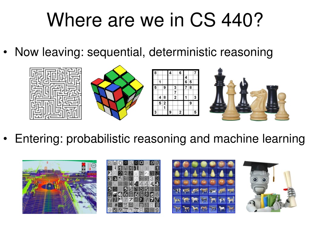
1. Where are we in CS 440? Now leaving: sequential, deterministic reasoning Entering: probabilistic reasoning and machine learning

2. Probability: Review of main concepts (Chapter 13)

3. Outline Motivation: Why use probability? Laziness, Ignorance, and Randomness Rational Bettor Theorem Review of Key Concepts Outcomes, Events, and Random Variables Joint, Marginal, and Conditional Independent Events

4. Outline Motivation: Why use probability? Laziness, Ignorance, and Randomness Rational Bettor Theorem Review of Key Concepts Outcomes, Events, and Random Variables Joint, Marginal, and Conditional Independence and Conditional Independence

5. Motivation: Planning under uncertainty Recall: representation for planning States are specified as conjunctions of predicates Start state: At(P1, CMI) Plane(P1) Airport(CMI) Airport(ORD) Goal state: At(P1, ORD) Actions are described in terms of preconditions and effects: Fly(p, source, dest) Precond: At(p, source) Plane(p) Airport(source) Airport(dest) Effect: At(p, source) At(p, dest)

6. Motivation: Planning under uncertainty Let action At= leave for airport t minutes before flight Will Atsucceed, i.e., get me to the airport in time for the flight? Problems: Partial observability (road state, other drivers' plans, etc.) Noisy sensors (traffic reports) Uncertainty in action outcomes (flat tire, etc.) Complexity of modeling and predicting traffic Hence a purely logical approach either Risks falsehood: A25will get me there on time, or Leads to conclusions that are too weak for decision making: A25will get me there on time if there's no accident on the bridge and it doesn't rain and my tires remain intact, etc., etc. A1440will get me there on time but I ll have to stay overnight in the airport

7. Probability Probabilistic assertions summarize effects of Laziness: reluctance to enumerate exceptions, qualifications, etc. Ignorance: lack of explicit theories, relevant facts, initial conditions, etc. Intrinsically random phenomena

8. Outline Motivation: Why use probability? Laziness, Ignorance, and Randomness Rational Bettor Theorem Review of Key Concepts Outcomes, Events, and Random Variables Joint, Marginal, and Conditional Independence and Conditional Independence

9. Making decisions under uncertainty Suppose the agent believes the following: P(A25gets me there on time) = 0.04 P(A90gets me there on time) = 0.70 P(A120 gets me there on time) = 0.95 P(A1440gets me there on time) = 0.9999 Which action should the agent choose? Depends on preferences for missing flight vs. time spent waiting Encapsulated by a utility function The agent should choose the action that maximizes the expected utility: P(Atsucceeds) * U(Atsucceeds) + P(Atfails) * U(Atfails)

10. Making decisions under uncertainty More generally: the expected utility of an action is defined as: EU(a) = outcomes of aP(outcome|a) U(outcome) Utility theory is used to represent and infer preferences Decision theory = probability theory + utility theory

11. Monty Hall problem You re a contestant on a game show. You see three closed doors, and behind one of them is a prize. You choose one door, and the host opens one of the other doors and reveals that there is no prize behind it. Then he offers you a chance to switch to the remaining door. Should you take it? http://en.wikipedia.org/wiki/Monty_Hall_problem

12. Monty Hall problem With probability 1/3, you picked the correct door, and with probability 2/3, picked the wrong door. If you picked the correct door and then you switch, you lose. If you picked the wrong door and then you switch, you win the prize. Expected utility of switching: EU(Switch) = (1/3) * 0 + (2/3) * Prize Expected utility of not switching: EU(Not switch) = (1/3) * Prize + (2/3) * 0

13. Where do probabilities come from? Frequentism Probabilities are relative frequencies For example, if we toss a coin many times, P(heads) is the proportion of the time the coin will come up heads But what if we re dealing with events that only happen once? E.g., what is the probability that Team X will win the Superbowl this year? Reference class problem Subjectivism Probabilities are degrees of belief But then, how do we assign belief values to statements? What would constrain agents to hold consistent beliefs?

14. The Rational Bettor Theorem Why should a rational agent hold beliefs that are consistent with axioms of probability? For example, P(A) + P( A) = 1 If an agent has some degree of belief in proposition A, he/she should be able to decide whether or not to accept a bet for/against A (De Finetti, 1931): If the agent believes that P(A) = 0.4, should he/she agree to bet $4 that A will occur against $6 that A will not occur? Theorem: An agent who holds beliefs inconsistent with axioms of probability can be convinced to accept a combination of bets that is guaranteed to lose them money

15. Outline Motivation: Why use probability? Laziness, Ignorance, and Randomness Rational Bettor Theorem Review of Key Concepts Outcomes, Events, and Random Variables Joint, Marginal, and Conditional Independence and Conditional Independence

16. Outcomes of an Experiment The SET OF POSSIBLE OUTCOMES (a.k.a. the sample space ) is a listing of all of the things that might happen: 1. Mutually exclusive. It s not possible that two different outcomes might both happen. 2. Collectively exhaustive. Every outcome that could possibly happen is one of the items in the list. 3. Finest grain. After the experiment occurs, somebody tells you the outcome, and there is nothing else you need to know. Example experiment: Alice, Bob, Carol and Duane run a 10km race to decide who will buy pizza tonight. Outcome = a listing of the exact finishing times of each participant.

17. Events Probabilistic statements are defined over events, or sets of world states A = It is raining B = The weather is either cloudy or snowy C = The sum of the two dice rolls is 11 D = My car is going between 30 and 50 miles per hour An EVENT is a SET of OUTCOMES B = { outcomes : cloudy OR snowy } C = { outcomes : d1+d2 = 11 } Notation: P(A) is the probability of the set of world states (outcomes) in which proposition A holds

18. Kolmogorovs axioms of probability For any propositions (events) A, B 0 P(A) 1 P(True) = 1 and P(False) = 0 P(A B) = P(A) + P(B) P(A B) Subtraction accounts for double-counting Based on these axioms, what is P( A)? These axioms are sufficient to completely specify probability theory for discrete random variables For continuous variables, need density functions

19. Outcomes = Atomic events OUTCOME or ATOMIC EVENT: is a complete specification of the state of the world, or a complete assignment of domain values to all random variables Atomic events are mutually exclusive and exhaustive E.g., if the world consists of only two Boolean variables Cavity and Toothache, then there are four outcomes: Cavity Toothache Cavity Toothache Cavity Toothache Cavity Toothache

20. Random variables We describe the (uncertain) state of the world using random variables Denoted by capital letters R: Is it raining? W:What s the weather? D: What is the outcome of rolling two dice? S: What is the speed of my car (in MPH)? Just like variables in CSPs, random variables take on values in a domain Domain values must be mutually exclusive and exhaustive R in {True, False} W in {Sunny, Cloudy, Rainy, Snow} D in {(1,1), (1,2), (6,6)} S in [0, 200]

21. Events and Outcomes An OUTCOME (ATOMIC EVENT) is a particular setting of all of the random variables Outcome = ( number rolled on die 1, number on die 2 ) An EVENT is a SET of OUTCOMES The sum of the two dice rolls is 11 = { set of all outcomes such that d1+d2 = 11 } P ????? = ???????? ? ??????(???????)

22. Outline Motivation: Why use probability? Laziness, Ignorance, and Randomness Rational Bettor Theorem Review of Key Concepts Outcomes, Events, and Random Variables Joint, Marginal, and Conditional Independence and Conditional Independence

23. Joint probability distributions A joint distribution is an assignment of probabilities to every possible atomic event Atomic event Cavity Toothache Cavity Toothache Cavity Toothache Cavity Toothache P 0.8 0.1 0.05 0.05 Why does it follow from the axioms of probability that the probabilities of all possible atomic events must sum to 1?

24. Joint probability distributions A joint distribution is an assignment of probabilities to every possible atomic event Suppose we have a joint distribution of n random variables with domain sizes d What is the size of the probability table? Impossible to write out completely for all but the smallest distributions

25. Notation P(X1 = x1, X2 = x2, , Xn = xn) refers to a single entry (atomic event) in the joint probability distribution table Shorthand: P(x1, x2, , xn) P(X1, X2, , Xn) refers to the entire joint probability distribution table P(A) can also refer to the probability of an event E.g., X1 = x1 is an event

26. Marginal probability distributions From the joint distribution P(X,Y) we can find the marginal distributions P(X) and P(Y) P(Cavity, Toothache) Cavity Toothache Cavity Toothache Cavity Toothache Cavity Toothache 0.8 0.1 0.05 0.05 P(Cavity) Cavity Cavity P(Toothache) Toothache Toochache ? ? ? ?

27. Marginal probability distributions From the joint distribution P(X,Y) we can find the marginal distributionsP(X) and P(Y) To find P(X = x), sum the probabilities of all atomic events where X = x: ( ) = = = = = = ( ) ( ) ( ) P X x P X x Y y X x Y y 1 n n ( ) = = ( , ) ( , ) ( , ) P x y x y P x y 1 n i = This is called marginalization (we are marginalizing out all the variables except X) 1 i

28. Conditional probability Probability of cavity given toothache: P(Cavity = true | Toothache = true) ( P ) ( P , B ) P A B P A B = = ( | ) P A B For any two events A and B, ( ) ( ) B P(A B) P(A) P(B)

29. Conditional probability P(Cavity, Toothache) Cavity Toothache Cavity Toothache Cavity Toothache Cavity Toothache 0.8 0.1 0.05 0.05 P(Cavity) Cavity Cavity P(Toothache) Toothache Toochache 0.9 0.1 0.85 0.15 What is P(Cavity = true | Toothache = false)? 0.05 / 0.85 = 0.059 What is P(Cavity = false | Toothache = true)? 0.1 / 0.15 = 0.667

30. Conditional distributions A conditional distribution is a distribution over the values of one variable given fixed values of other variables P(Cavity, Toothache) Cavity Toothache Cavity Toothache Cavity Toothache Cavity Toothache 0.8 0.1 0.05 0.05 P(Cavity | Toothache = true) Cavity Cavity P(Cavity|Toothache = false) Cavity Cavity 0.667 0.333 0.941 0.059 P(Toothache | Cavity = true) Toothache Toochache P(Toothache | Cavity = false) Toothache Toochache 0.5 0.5 0.889 0.111

31. Normalization trick To get the whole conditional distribution P(X | Y = y) at once, select all entries in the joint distribution table matching Y = y and renormalize them to sum to one P(Cavity, Toothache) Cavity Toothache Cavity Toothache Cavity Toothache Cavity Toothache 0.8 0.1 0.05 0.05 Select Toothache, Cavity = false Toothache Toochache 0.8 0.1 Renormalize P(Toothache | Cavity = false) Toothache Toochache 0.889 0.111

32. Normalization trick To get the whole conditional distribution P(X | Y = y) at once, select all entries in the joint distribution table matching Y = y and renormalize them to sum to one Why does it work? ( P , x ) ( , y ) P x y P x y = by marginalization ( , ) ( ) y P x

33. Product rule ( P , B ) P A B = ( | ) P A B Definition of conditional probability: ( ) Sometimes we have the conditional probability and want to obtain the joint: = = ( , ) ( | ) ( ) ( | ) ( ) P A B P A B P B P B A P A

34. Product rule ( P , B ) P A B = ( | ) P A B Definition of conditional probability: ( ) Sometimes we have the conditional probability and want to obtain the joint: = = ( , ) ( | ) ( ) ( | ) ( ) P A B P A B P B P B A P A The chain rule: = ( , , ) ( ) ( | ) ( | , ) ( | , , ) P A A P A P A A P A A A P A A A 1 1 2 1 3 1 2 1 1 n n n n = i = ( | , , ) P A A A 1 1 i i 1

35. The Birthday problem We have a set of n people. What is the probability that two of them share the same birthday? Easier to calculate the probability that n people donot share the same birthday ( P , B distinct ) P B B 1 n = ( distinct B from , | , distinct ) B B B B 1 1 1 1 n n n ( , distinct ) P = i B 1 1 n n = ( distinct from , | , distinct ) P B B B B B 1 1 1 1 i i i 1

36. The Birthday problem ( , distinct ) P B B 1 n n = i = ( distinct from , | , distinct ) P B B B B B 1 1 1 1 i i i 1 i + 365 1 = ( distinct from , , | , , distinct) P B B B B B 1 1 1 1 i i i 365 + 365 364 365 1 n = ( , , distinct) P B B 1 n 365 365 365 + 365 364 365 1 n = ( , , distinct) not 1 P B B 1 n 365 365 365

37. The Birthday problem For 23 people, the probability of sharing a birthday is above 0.5! http://en.wikipedia.org/wiki/Birthday_problem

38. Outline Motivation: Why use probability? Laziness, Ignorance, and Randomness Rational Bettor Theorem Review of Key Concepts Outcomes, Events, and Random Variables Joint, Marginal, and Conditional Independence and Conditional Independence

39. Independence Two events A and B are independent if and only if P(A B) = P(A, B) = P(A) P(B) In other words, P(A | B) = P(A) and P(B | A) = P(B) This is an important simplifying assumption for modeling, e.g., Toothache and Weather can be assumed to be independent Are two mutually exclusive events independent? No, but for mutually exclusive events we have P(A B) = P(A) + P(B)

40. Independence Two events A and B are independent if and only if P(A B) = P(A) P(B) In other words, P(A | B) = P(A) and P(B | A) = P(B) This is an important simplifying assumption for modeling, e.g., Toothache and Weather can be assumed to be independent Conditional independence: A and B are conditionally independent given C iff P(A B | C) = P(A | C) P(B | C) Equivalently: P(A | B, C) = P(A | C) or P(B | A, C) = P(B | C)

41. Conditional independence: Example Toothache: boolean variable indicating whether the patient has a toothache Cavity: boolean variable indicating whether the patient has a cavity Catch: whether the dentist s probe catches in the cavity If the patient has a cavity, the probability that the probe catches in it doesn't depend on whether he/she has a toothache P(Catch | Toothache, Cavity) = P(Catch | Cavity) Therefore, Catch is conditionally independent of Toothache given Cavity Likewise, Toothache is conditionally independent of Catch given Cavity P(Toothache | Catch, Cavity) = P(Toothache | Cavity) Equivalent statement: P(Toothache, Catch | Cavity) = P(Toothache | Cavity) P(Catch | Cavity)

42. Conditional independence: Example How many numbers do we need to represent the joint probability table P(Toothache, Cavity, Catch)? 23 1 = 7 independent entries Write out the joint distribution using chain rule: P(Toothache, Catch, Cavity) = P(Cavity) P(Catch | Cavity) P(Toothache | Catch, Cavity) = P(Cavity) P(Catch | Cavity) P(Toothache | Cavity) How many numbers do we need to represent these distributions? 1 + 2 + 2 = 5 independent numbers In most cases, the use of conditional independence reduces the size of the representation of the joint distribution from exponential in n to linear in n