Evolution of Robot Localization: From Deterministic to Probabilistic Approaches
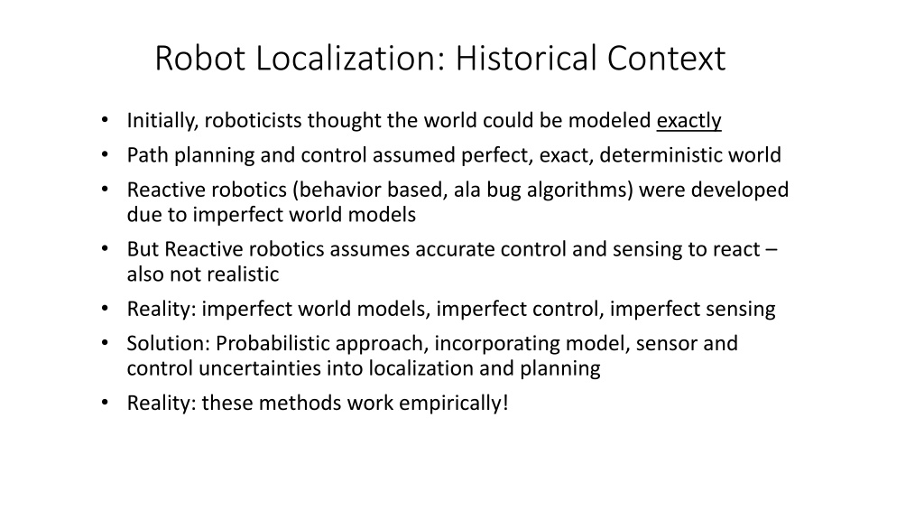
Roboticists initially aimed for precise world modeling leading to perfect path planning and control concepts. However, imperfections in world models, control, and sensing called for a shift towards probabilistic methods in robot localization. This evolution from reactive to probabilistic robotics has proven effective empirically, emphasizing the importance of incorporating uncertainties in modeling, sensing, and control for successful localization and planning in robotic systems.

Download Presentation

Please find below an Image/Link to download the presentation.
The content on the website is provided AS IS for your information and personal use only. It may not be sold, licensed, or shared on other websites without obtaining consent from the author. Download presentation by click this link. If you encounter any issues during the download, it is possible that the publisher has removed the file from their server.
E N D
Presentation Transcript
Robot Localization: Historical Context Initially, roboticists thought the world could be modeled exactly Path planning and control assumed perfect, exact, deterministic world Reactive robotics (behavior based, ala bug algorithms) were developed due to imperfect world models But Reactive robotics assumes accurate control and sensing to react also not realistic Reality: imperfect world models, imperfect control, imperfect sensing Solution: Probabilistic approach, incorporating model, sensor and control uncertainties into localization and planning Reality: these methods work empirically!
Map Learning and High Speed Navigation in RHINO Sebastian Thrun, Arno B ucken Wolfram Burgard Dieter Fox,Thorsten Fr ohlinghaus Daniel Hennig Thomas Hofmann Michael Krell Timo Schmidt An indoor mobile robot that uses sonar and vision to map its environment in real-time
Case Study: Map Learning and High Speed Navigation in RHINO Control is distributed and decentralized. Onboard and offboard machines are dedicated to several subproblems of modeling and control. Communication between modules is asynchronous - no central clock, and no central process controlller. Whenever possible, anytime algorithms are employed to ensure that the robot operates in realtime. Hybrid architecture. Fast, reactive mechanisms are integrated with computationally intense, deliberative modules. Models, such as the two dimensional maps described below, are used at all levels of architecture. Whenever possible, models are learned from data. Machine learning algorithms are employed to increase the flexibility and the robustness of the system. Learning has proven most useful close to the sensory side of the system, where algorithms such as artificial neural networks interpret the robot s sensors. Software is modular. A plug and play architecture allows us to quickly reconfigure the system, depending on the particular configuration and application. Sensor fusion. To maximize the robustness of the approach, most of the techniques described here rely on more than just a single type of sensor.
Requirements of a Map Representation for a Mobile Robot The precision of the map needs to match the precision with which the robot needs to achieve its goals The precision and type of features mapped must match the precision of the robot s sensors The complexity of the map has direct impact on computational complexity for localization, navigation and map updating
Mapping: Occupancy Grids 2D metric occupancy grids are used Each grid cell has probability of the cell being occupied, Prob(occ(x,y)) Occupancy grid integrates multiple sensors (e.g. sonar and stereo)
Sonar Data Interpretation Need to translate sonar distances into occupancy values: Prob(occ(x,y)) Method: Neural Net, trained on sonar responses RHINO uses a 360 ring of sonars Input to net: 4 readings nearest (x,y) encoded as polar coordinates Output: Prob(occ(x,y)) Training data: train with physical robot on real known environments or use robot simulator May need to train anew in different environments wall textures etc. Key point: multiple spatial readings needed to overcome noise and sonar effects
Sonar scan Probabilistic Occupancy Grid
Stereo Data Interpretation Vertical edges (doorways, vertical corners, obstacles) are found in each image and triangulated for 3D depth. 3D edge points are projected onto the occupancy grid after being enlarged by the robot radius Enlargement allows robot to navigate without hitting corners Stereo can miss featureless, homogeneous areas like blank walls Integration with sonar can improve mapping accuracy
Vertical edges image Vertical edge projection Occupancy grid Results from Stereo matching
Updating over time Mobile robot is moving and making multiple measurements at each sensing time step Need to integrate the new values from the sensors with the current occupancy grid values These are probabilistic measures, so a Bayes rule update is used to find new probability of occupancy (more on this later .)
Integration results Maps built in a single run (a) using only sonar sensors, (b) using only stereo information, and (c) integrating both. Notice that sonar models the world more consistently, but misses the two sonar absorbing Chairs which are found using stereo vision.
Topological Maps Compact representation, usually as a graph Nodes are distinct places, arcs (edges) represent adjacency Regions of free-space are nodes, and edges represent connections for adjacency Method: Create Voronoi diagram Find critical points bottlenecks or choke points in the Voronoi diagram Formally, a threshold epsilon for minimum distance to obstacle locally Find critical lines: partitions between regions at bottlenecks Partitions are used to form a graph. Nodes are regions, arcs are adjacent regions separated by critical lines
Voronoi Diagram Critical points Topological map Regions
Path Planning More on this later for now suffice to use a graph search from a start region on the map to a goal region.
TopBot: Topological Mobile Robot Localization Using Fast Vision Techniques Paul Blaer and Peter Allen Dept. of Computer Science, Columbia University {psb15, allen}@cs.columbia.edu
Autonomous Vehicle for Exploration and Navigation in Urban Environments GPS The AVENUE Robot: Autonomous. Operates in outdoor urban environments. Builds accurate 3-D models. Scanner DGPS Network Camera PTU Current Localization Methods: Odometry. Differential GPS. Vision. Compass Sonars PC
Main Vision System Georgiev and Allen 02
Topological Localization Odometry and GPS can fail. Fine vision techniques need an estimate of the robot s current position. ------------------------------------------ Histogram Matching of Omnidirectional Images: Fast. Rotationally-invariant. Finds the region of the robot. This region serves as a starting estimate for the main vision system. Omnidirectional Camera
Related Work Omnidirectional Imaging for Navigation. Ulrich and Nourbakhsh 00 (with histogramming); Cassinis et al. 96; Winters et al. 00. Topological Navigation. Kuipers and Byun 91; Radhakrishnan and Nourbakhsh 99. Other Approaches to Robot Localization. Castellanos et al. 98; Durrant-Whyte et al. 99; Leonard and Feder 99; Thrun et al. 98; Dellaert et al. 99; Simmons and Koenig 95. ------------------------------------------------------------------------------------------ AVENUE Allen, Stamos, Georgiev, Gold, Blaer 01.
Building the Database Divide the environment into a logical set of regions. Reference images must be taken in all of these regions. The images should be taken in a zig-zag pattern to cover as many different locations as possible. Each image is reduced to three 256-bucket histograms, for the red, green, and blue color bands.
An Image From the Omnidirectional Camera
Masking the Image The camera points up to get a clear picture of the buildings. The camera pointing down would give images of the ground s brick pattern - not useful for histogramming. With the camera pointing up, the sun and sky enter the picture and cause major color variations. We mask out the center of the image to block out most of the sky. We also mask out the superstructure associated with the camera.
Environmental Effects Indoor environments Controlled lighting conditions No histogram adjustments Outdoor environments Large variations in lighting Use a histogram normalization with the percentage of color at each pixel: R + + G B , , + + + + R G B R G B R G B
Indoor Image Non-Normalized Histogram
Outdoor Image Normalized Histogram
Matching an Unknown Image with the Database Compare unknown image to each image in the database. Initially we treat each band (r, g, b) separately. The difference between two histograms is the sum of the absolute differences of each bucket. Better to sum the differences for all three bands into a single metric than to treat each band separately. The region of the database image with the smallest difference is the selected region for this unknown.
Image Matching to the Database Histogram Difference Database Image
The Test Environments Indoor Outdoor (Aerial View) Outdoor (Campus Map) (Hallway View)
Indoor Results Images Tested 21 12 9 5 23 9 5 5 89 Non-Normalized % Correct 100% 83% 77% 20% 74% 89% 0% 100% 78% Normalized % Correct 95% 92% 89% 20% 91% 78% 20% 40% 80% Region 1 2 3 4 5 6 7 8 Total
Ambiguous Regions South Hallway North Hallway
Outdoor Results Images Tested 50 50 50 50 50 50 50 50 400 Non-Normalized % Correct 58% 11% 29% 25% 49% 30% 28% 41% 34% Normalized % Correct 95% 39% 71% 62% 55% 57% 61% 78% 65% Region 1 2 3 4 5 6 7 8 Total
The Best Candidate Regions Histogram Difference Wrong Region, Second-Lowest Difference Correct Region, Lowest Difference Database Image
Conclusions In 80% of the cases we were able to narrow down the robot s location to only 2 or 3 possible regions without any prior knowledge of the robot s position. Our goal was to reduce the number of possible models that the fine- grained visual localization method needed to examine. Our method effectively quartered the number of regions that the fine-grained method had to test.
Future Work What is needed is a fast secondary discriminator to distinguish between the 2 or 3 possible regions. Histograms are limited in nature because of their total reliance on the color of the scene. To counter this we want to incorporate more geometric data into our database, such as edge images.