Understanding Power, Type I Error, and FDR in Statistical Genomics
Explore concepts of statistical genomics in Lecture 11 focusing on power, type I error, and false discovery rate (FDR) in GWAS analysis. The content covers simulations of phenotype from genotype data, GWAS by correlation, resolution and bin approach, and implications on QTN bins for power and error rates. Gain insights into interpreting results and distinguishing between true and false discoveries in genomic studies.

Uploaded on Oct 06, 2024 | 0 Views
Download Presentation

Please find below an Image/Link to download the presentation.
The content on the website is provided AS IS for your information and personal use only. It may not be sold, licensed, or shared on other websites without obtaining consent from the author. Download presentation by click this link. If you encounter any issues during the download, it is possible that the publisher has removed the file from their server.
E N D
Presentation Transcript
Statistical Genomics Statistical Genomics Lecture 11: Power, type I error and FDR Lecture 11: Power, type I error and FDR Zhiwu Zhang Washington State University
Outline Simulation of phenotype from genotype GWAS by correlation Power FDR Cutoff Null distribution of p values Resolution QTN bins and non-QTN bins
GWAS by correlation GWAS by correlation myGD=read.table(file="http://zzlab.net/GAPIT/data/mdp_numeric.txt",head=T) myGM=read.table(file="http://zzlab.net/GAPIT/data/mdp_SNP_information.txt",head=T) source("http://zzlab.net/StaGen/2020/R/G2P.R") source("http://zzlab.net/StaGen/2020/R/GWASbyCor.R") X=myGD[,-1] set.seed(99164) mySim=G2P(X= myGD[,-1],h2=.75,alpha=1,NQTN=10,distribution="normal") p= GWASbyCor(X=X,y=mySim$y) color.vector <- rep(c("deepskyblue","orange","forestgreen","indianred3"),10) m=nrow(myGM) plot(t(-log10(p))~seq(1:m),col=color.vector[myGM[,2]]) abline(v=mySim$QTN.position, lty = 2, lwd=2, col = "black") 15 t(-log10(p)) 10 5 0 0 500 1000 1500 2000 2500 3000 seq(1:m)
Resolution and bin approach Resolution and bin approach 10Kb is really good, 100Kb is OK Bins with QTNs for power Bins without QTNs for type I error
Bins (e.g. 100Kb) Bins (e.g. 100Kb) bigNum=1e9 resolution=100000 bin=round((myGM[,2]*bigNum+myGM[,3])/resolution) result=cbind(myGM,t(p),bin) head(result) Minimum p value within bin
Bins of QTNs Bins of QTNs QTN.bin=result[mySim$QTN.position,] QTN.bin
Sorted bins of QTNs Sorted bins of QTNs index.qtn.p=order(QTN.bin[,4]) QTN.bin[index.qtn.p,]
FDR and type I error FDR and type I error Total number of bins: 3054 (size of 100kb) N 1 2 3 4 5 6 7 8 9 10 bin 50120 12235 60985 12918 31482 101348 31573 42222 10502 22331 t(p) 4.44E-16 1.00E-10 1.38E-10 7.02E-08 2.05E-05 9.58E-02 1.88E-01 2.94E-01 4.98E-01 9.91E-01 Power 0.1 0.2 0.3 0.4 0.5 0.6 0.7 0.8 0.9 1 #False bins 0 0 0 0 2 416 608 782 1001 1335 FDR 0 0 0 0 TypeI Error 0 0 0 0 0.000654879 0.1362148 0.19908317 0.256057629 0.327766863 0.437131631 0.285714286 0.985781991 0.988617886 0.989873418 0.991089109 0.992565056 0.285714286=2/(2+5) 0.000654879=2/3054
ROC curve ROC curve Receiver Operating Characteristic "The curve is created by plotting the true positive rate against the false positive rate at various threshold settings." -Wikipedia Power FDR Liu et. al. PLoS Genetics, 2016
GAPIT.FDR.TypeI GAPIT.FDR.TypeI Function Function library(compiler) #required for cmpfun source("http://www.zzlab.net/GAPIT/gapit_functions.txt") myStat=GAPIT.FDR.TypeI( WS=c(1e0,1e3,1e4,1e5), GM=myGM, seqQTN=mySim$QTN.position, GWAS=result) str(myStat)
Return Return
Area Under Curve (AUC) Area Under Curve (AUC) par(mfrow=c(1,2),mar = c(5,2,5,2)) plot(myStat$FDR[,1],myStat$Power,type="b") plot(myStat$TypeI[,1],myStat$Power,type="b") 1.0 1.0 0.8 0.8 0.6 0.6 0.4 0.4 0.2 0.2 0.0 0.2 0.4 0.6 0.8 1.0 0.0 0.2 0.4 0.6 0.8 myStat$FDR[, 1] myStat$TypeI[, 1]
Replicates Replicates nrep=100 set.seed(99164) statRep=replicate(nrep, { mySim=G2P(X=myGD[,-1],h2=.5,alpha=1,NQTN=10,distribution="norm") p=p= GWASbyCor(X=myGD[,-1],y=mySim$y) seqQTN=mySim$QTN.position myGWAS=cbind(myGM,t(p),NA) myStat=GAPIT.FDR.TypeI(WS=c(1e0,1e3,1e4,1e5), GM=myGM,seqQTN=mySim$QTN.position,GWAS=myGWAS,maxOut=100, MaxBP=1e10) })
str str( (statRep statRep) )
Means over replicates Means over replicates power=statRep[[2]] #FDR s.fdr=seq(3,length(statRep),7) fdr=statRep[s.fdr] fdr.mean=Reduce ("+", fdr) / length(fdr) #AUC: power vs. FDR s.auc.fdr=seq(6,length(statRep),7) auc.fdr=statRep[s.auc.fdr] auc.fdr.mean=Reduce ("+", auc.fdr) / length(auc.fdr)
Plots of power vs. FDR Plots of power vs. FDR theColor=rainbow(4) plot(fdr.mean[,1],power , type="b", col=theColor [1],xlim=c(0,1)) for(i in 2:ncol(fdr.mean)){ lines(fdr.mean[,i], power , type="b", col= theColor [i]) } 1.0 0.8 0.6 power 0.4 0.2 0.0 0.2 0.4 0.6 0.8 1.0 fdr.mean[, 1]
Plots of AUC Plots of AUC barplot(auc.fdr.mean, names.arg=c("1bp", "1K", "10K","100K"), xlab="Resolution", ylab="AUC") 0.30 0.20 AUC 0.10 0.00 1bp 1K 10K 100K Resolution
ROC with different heritability ROC with different heritability h2= 25% vs. 75% 10 QTNs Normal distributed QTN effect 100kb resolution Power against Type I error
Simulation and GWAS Simulation and GWAS nrep=100 set.seed(99164) #h2=25% statRep25=replicate(nrep, { mySim=G2P(X=myGD[,-1],h2=.25,alpha=1,NQTN=10,distribution="norm") p=p= GWASbyCor(X=myGD[,-1],y=mySim$y) seqQTN=mySim$QTN.position myGWAS=cbind(myGM,t(p),NA) myStat=GAPIT.FDR.TypeI(WS=c(1e0,1e3,1e4,1e5), GM=myGM,seqQTN=mySim$QTN.position,GWAS=myGWAS,maxOut=100,MaxBP=1e10)}) #h2=75% statRep75=replicate(nrep, { mySim=G2P(X=myGD[,-1],h2=.75,alpha=1,NQTN=10,distribution="norm") p= GWASbyCor(X=myGD[,-1],y=mySim$y) seqQTN=mySim$QTN.position myGWAS=cbind(myGM,t(p),NA) myStat=GAPIT.FDR.TypeI(WS=c(1e0,1e3,1e4,1e5), GM=myGM,seqQTN=mySim$QTN.position,GWAS=myGWAS,maxOut=100,MaxBP=1e10)})
Means and plot Means and plot power25=statRep25[[2]] s.t1=seq(4,length(statRep25),7) t1=statRep25[s.t1] t1.mean.25=Reduce ("+", t1) / length(t1) power75=statRep75[[2]] s.t1=seq(4,length(statRep75),7) t1=statRep75[s.t1] t1.mean.75=Reduce ("+", t1) / length(t1) plot(t1.mean.25[,4],power25, type="b", col="blue",xlim=c(0,0.6)) lines(t1.mean.75[,4], power75, type="b", col= "red")
Outline Simulation of phenotype from genotype GWAS by correlation Power FDR Cutoff Null distribution of p values Resolution QTN bins and non-QTN bins


")


")