Dynamic Behavior Modeling of Manufacturing Systems using Petri Nets
Introduction to Petri nets and their application in modeling manufacturing systems. Covers formal definitions, elementary classes, properties, and analysis methods of Petri net models. Explores a two-product system example and its process modeling with shared and dedicated resources.

Download Presentation

Please find below an Image/Link to download the presentation.
The content on the website is provided AS IS for your information and personal use only. It may not be sold, licensed, or shared on other websites without obtaining consent from the author. Download presentation by click this link. If you encounter any issues during the download, it is possible that the publisher has removed the file from their server.
E N D
Presentation Transcript
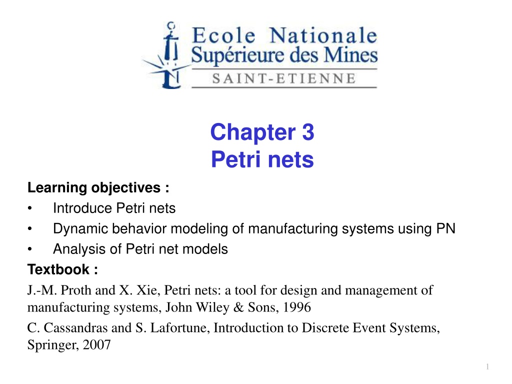
Chapter 3 Petri nets Learning objectives : Introduce Petri nets Dynamic behavior modeling of manufacturing systems using PN Analysis of Petri net models Textbook : J.-M. Proth and X. Xie, Petri nets: a tool for design and management of manufacturing systems, John Wiley & Sons, 1996 C. Cassandras and S. Lafortune, Introduction to Discrete Event Systems, Springer, 2007 1
Plan Introduction to Petri nets Formal definitions Petri net models of manufacturing system Elementary classes of Petri nets Properties of PN models Analysis methods 2 2
A two-product system Two types P1 and P2 of products are produced. The production of each product requires two operations. The first operation is performed by a shared machine. The second operation is performed by a dedicated machine. There is at most one product of each type loaded in the system at any time. When a product finishes, a new product of the same type is dispatched. To be modelled using an usual process-resource modelling approach. 4
A two-product system Process modeling Goal: model the manufacturing process of each product, i.e. all possible states of a product including waiting Identify all relevant operations and their precedence constraints. Identify all possible waits for shared resources. 5
A two-product system Process : P1, P2 Resource : M (shared machine) Dedicated machines are not restrictive resources here (Why) Process steps : Step 0 1 2 Meaning Ready and wait for M Operation on M Operation on dedicated machine 1 Res. Requirement P1 M - Step 0 1 2 Meaning Ready and wait for M Operation on M Operation on dedicated machine 2 Res. Requirement P2 M - 6
A two-product system Process modeling Associate each process a state-transition graph. wait for shared machine p1 p4 t1 t4 parts under operation 1 p2 p5 t2 t5 parts under operation 2 p3 p6 t3 t6 7
A two-product system Process modelling Goal: model the manufacturing process of each product. Include eventual constraints related to production control. There is at most one product of each type loaded in the system at any time. p1 p4 t1 t4 p2 p5 t2 t5 p3 p6 t3 t6 8
A two-product system Resource modelling Goal: modelling resource contraint + eventual priority constraints Identifies p1 p4 t1 t4 p7 transitions after which the resource is first needed p2 p5 M t2 t5 p3 p6 transitions after which the resource is no longer needed t3 t6 P2 P1 9
Places and transitions A PETRI NET is a bipartite graph which consists of two types of nodes: places and transitions connected by directed arcs. Place = circle, transition = bar or box. t4 p2 t2 p4 An arc connects a place to a transition or a transition to a place. p1 p3 t1 t3 No arcs between nodes of the same type. p5 t5 Input and output places of a transition Input and output transitions of a place
Token and marking system state Each place contains a number of tokens. The distribution of tokens in the Petri net is called the marking. Representations of a marking: a vector M = (m1, m2, , mn) where mi = nb of tokens in place pi a multi-set such as M = p1 2p3 The marking of an PN = state of the corresponding system. t4 p2 t2 p4 p1 The initial state of the system = the initial marking, denoted as M0. p3 t1 t3 p5 t5 Example: M = ( ???) = ??? 11
System dynamics by transition firing A transition is said enabled (firable) if each of its input places contains at least one token. An enabled transition can fire. Firing a transition removes a token from each input place and add one token to each ouput place. Firing a transition leads to a new marking that enables other transitions. The dynamic behavior of the corresponding system = evolution of the marking and transition firings Convention: simultaneous transition firings are forbidden. 12
Sequence of transitions A sequence of transitions that can be fired consecutively starting from the initial marking is said enabled or firable. The sequence of firable transitions is not unique. The set of all firable sequences of transitions = PN language Example: sequence t1t2t1t3 t4 p2 t2 p4 p1 p3 t1 t3 p5 t5 14
Petri Nets A Petri net is a five-tuple PN = (P, T, A, W, M0) where: P = { p1, p2, ..., pn} is a finite set of places T = { t1, t2, ..., tm } is a finite set of transitions A (P T) (T P) is a set of arcs W : A { 1, 2, ... } is a weight function M0 : P { 0, 1, 2, ... } is the initial marking P T = and P T = PN without the initial marking is denoted by N: N = (P, T, A, W) PN = (N, M0) A Petri net is said ordinary if w(a) = 1, a A. 16
Graphic representation Similar to that of ordinary PN but with default weight of 1 when not explicitly represented. t4 p2 t2 p4 p1 2 p3 t1 t3 p5 t5 17
Transition firing Rule 1: A transition t is enabled at a marking M if M (p) w(p, t) for any p ot whereot is the set of input places of t Rule 2: An enabled transition may or may not fire. Rule 3: Firing transition t results in: removing w(p, t) tokens from each p ot adding w(t, p) tokens to each p to where to is the set of output places of t M(t> M' denotes firing t at marking M with M p ( ), M p ( )+ W t,p M p ( ) W p,t M p ( )+ W t,p si (p,t) A et (t,p) A, si (p,t) A et (t,p) A, si (p,t) A et (t,p) A, si (p,t) A et (t,p) A, ( ( ( ), ), ) W p,t M' p ( )= ( ),
Transition firing 2 2 2 2 2 2 2 2 19
Basic concepts Source transition: transition without input places, i.e. ot = . Sink transition: transition without output places, i.e. to= . Source place: place without input transitions, i.e. op = . Sink place: place without output transitions, i.e. po= . Self-loop: a couple (p, t) such that t is both input and output transition of p Path: a sequence of nodes s1s2 snsuch that si+1is an output node of si. Circuit: a path such that sn= s1. Online illustration
Basic concepts t5 p1 5 Source transition t5 p6 p0 Sink transition t10 t1 t6 Source place p1 p2 p7 Sink place p5 t2 t7 r2 r1 p3 p8 Self-loop t3 t8 Path p4 p9 Circuit t4 t9 p5 p10 t10
Incidence matrices Pre incidence matrix: ( ) , , if w p t p t ( ) = Pre , p t 0, otherwise Post incidence matrix: ( ) , , if w t p p t ( ) = Post , p t 0, otherwise Incidence matrix : C = Post Pre. C(., t) = Token flow balance after firing t Pre and Post define the Petri net For Petri nets without self-loops, i.e. ot to= , C defines the Petri net with Pre(p,t) = max{0, C(p,t)} and Post(p,t) = max{0, C(p,t)}
Incidence matrices Example: Pre = ???, Post = ???, C = ??? t4 p2 t2 p4 p1 2 p3 t1 t3 p5 t5
Incidence matrices Enabled transition: A transition t is enabled at a marking M if M Pre( , t) Transition firing: Firing a transition t at marking M leads to M = M + C( , t) Sequence of transitions: Firing a sequence = t1t2 tn of transition starting from marking M leads to: ' M M C = + (1) where is the counting vector of the sequence . (proof) Equation (1) is also called state equation . Question: can this equation be used to checked the feasibility of a sequence and the reachability of a marking?
Incidence matrices Example: Markings after = t1t5t2t3t5 t4 p2 t2 p4 p1 2 p3 t1 t3 p5 t5 Observe the state equation of = t5t5t1t2t3. What conclusion?
PN models of key characteristics Parallel processes: Precedence relation: parallel process End Start start Activity2 End Activity1 Alternative processes: Synchronization: Alternattive process Waiting Sync Start End 27
PN models of key characteristics Buffer of finite capacity (4): pv Part arrival Part request pb FIFO system: 28
PN models of key characteristics Shared resources: Process with Resource Other Activities Waiting for Resource p1 r p2 29
PN models of key characteristics Shared machine: Dedicated machine: 30
PN models of key characteristics Unreliable machines: Assembly operation: pf output buffer capacity n1 Input buffer pw n2 pb pr 31
A robotic cell I Z1 M1 t1 M1 P1 S t2 Robot Unload M2 T Stock R n Q load t3 P2 t4 M2 Z2 32 O
A two-product system Two types P1 and P2 of products are produced. The production of each product requires two operations. The first operation is performed by a shared machine. The second operation is performed by a dedicated machine. There is at most one product of each type loaded in the system at any time. When a product finishes, a new product of the same type is dispatched. To be modelled using an usual process-resource modelling approach. 33
Process modeling Goal: model the manufacturing process of each product. Identify all relevant operations and their precedence constraints. Identify all possible waits for shared resources. wait for shared machine p1 p4 t1 t4 parts under operation 1 p2 p5 t2 t5 parts under operation 2 p3 p6 t3 t6 34
Process modelling Goal: model the manufacturing process of each product. Include eventual constraints related to production control. p1 p4 t1 t4 p2 p5 t2 t5 p3 p6 t3 t6 35
Resource modelling Goal: modelling resource contraint. Identifies p1 p4 t1 t4 p7 transitions after which the resource is first needed p2 p5 t2 t5 p3 p6 transitions after which the resource is no longer needed t3 t6 36
Pure Petri nets Definition: A Petri net free of self loop is said pure, i.e. ot to = . Theorem : All impure Petri nets can be transformed into pure Petri nets. p1 p1 b1 t1 e1 Sequential firing p0 p2 p2 b2 t2 e2 38
Ordinary Petri nets EVENT GRAPHS (OR MARKED GRAPHS) Each place has exactly one input and one output transition. STATE MACHINES Each transition has exactly one input place and one output place. Property: The total number of tokens in each elementary circuit is constant Property: The total number of token is constant. choice p1 t2 t1 synchronization t3 p3 t4 p2 39
Ordinary Petri nets FREE-CHOICE NETS card(p ) > 1 (p ) = {p}, p P EXTENDED FREE-CHOICE NETS p1 p2 p1 = p2 , p1, p2 P Can be transformed into a free-choice net. Property: Conflicting transitions are either all enabled or all not enabled. 40
Ordinary Petri nets ASYMMETRIC CHOICE NETS p1 p2 p1 p2 or p2 p1 , p1, p2 P Property : The set {p1, p2, , pk} of input places of any transition can be renumbered such that p1 p2 pk . p1 p3 p3 vs r r used by more transitions r p2 41
Relations between different classes PN = Petri Net AC = Assymmetric choice EFC = Extended Free Choice FC = Free Choice SM = State Machine EG = Event Graph FC PN EG SM AC EFC Ord. PN Conflict asym. choice SM AC Modeling power noEG noEFC sync. para. Confusion EG PN noSM Symmet. Choice noAC EFC 42 noFC
Reachability Reachable marking: A marking M is said reachable from another marking M if there exists a seqence of transitions such that M ( >M. Reachable set: R(M0) = set of markings reachable from the initial marking M0. Reachability is important for verification of the reachability of some desired (proper termination) or undesired markings (deadlock). Example: R(M0) = {(1, 0, 0, 0), (0, 1, 0, 0), (0, 0, 1, 0), (0, 0, 0, 1)} but (1, 0, 1, 0) not reachable. p1 : t1 p2 t3 Reachability = Petri net language t2 p3 t4 t5 44 p4
Reachability Theorem1 (monotonicity) : Any sequence of transitions firable starting from a marking M0 is also firable starting from M0 such that M0' M0. Theorem2 (necessary condition) : The equation system CY = M - M0 with Y 0 has a solution for all reachable marking M. Theorem3 (Acyclic PN) : For any PN free of cycles, a marking M is reachable iff the equation system C Y = M - M0with Y 0 has a solution. Ex: Find a PN and a marking that is not reachable but for which condition of Theorem 2 holds. 45
Boundedness A place p is said k-bounded if the number of tokens in p never exceed k, i.e. M(p) k, M R(M0). A Petri net is said k-bounded if all places are k-bounded, i.e. M(p) k, p and M R(M0). A Petri net is said bounded if it is k-bounded for some k > 0. A Petri net is said safe if it is 1-bounded, M(p) 1, p and M R(M0). Boundedness is often needed for a well-designed system as, without this property, goods could accumulated without limit, which is often a design error. 46
Boundedness p p p' 47
Boundedness Theorem (monotonicity) : If (N, M0) is bounded, then (N, M0 ) such that M0' M0 is bounded. Theorem (sufficient condition) : A Petri net (N, M0) is k-bounded if M(p) k, p and M such that M = M0 + CY for some Y 0. 48
Liveness A transition t is said live if it can always be made enabled starting from any reachable marking, i.e. M R(M0), M' R(M) such that M (t>. A Petri net is said live if all transitions are live. A transition is said quasi live if it can be fired at least once, i.e. M R(M0) such that M(t>. A Petri net is said quasi live if all transitions are quasi live. A marking M is said a deadlock or dead marking if no transition is enabled at M. A Petri net is said deadlock-free if it does not contain any deadlock. 49
Liveness Liveness implies the absence of total or partial deadlock and is often required for well-designed systems. But the reverse is not true. Deadlock often results from resource sharing and synchronization of parallel processes. No monotonicity of liveness as the Petri net below is not live if M0(R1) = 0, live if M0(R1) = 1, and not live if M0(R1) = 2. S1 S2 R1 S1 S2 R1 PN1 R3 PN2 R3 R2 R2 50