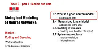
Exploring 2D Neuron Models and Phase Plane Analysis

Dive into the transition from Hodgkin-Huxley to 2D neuron models, understanding phase plane analysis, and analyzing different neuron types like Type I and II models with a focus on limit cycles, firing threshold, and separation of time scales.

Download Presentation

Please find below an Image/Link to download the presentation.
The content on the website is provided AS IS for your information and personal use only. It may not be sold, licensed, or shared on other websites without obtaining consent from the author. Download presentation by click this link. If you encounter any issues during the download, it is possible that the publisher has removed the file from their server.
E N D
Presentation Transcript
Week 4: Reducing Detail 2D models-Adding Detail 3.1 From Hodgkin-Huxley to 2D 3.2 Phase Plane Analysis 3.3 Analysis of a 2D Neuron Model 4.1 Type I and II Neuron Models - limit cycles - where is the firing threshold? - separation of time scales 4.2. Adding Detail - synapses -dendrites - cable equation Biological Modeling of Neural Networks Week 4 Reducing detail - Adding detail Wulfram Gerstner EPFL, Lausanne, Switzerland
Neuronal Dynamics Review from week 3 -Reduction of Hodgkin-Huxley to 2 dimension -step 1: separation of time scales -step 2: exploit similarities/correlations
Neuronal Dynamics 4.1. Reductionof Hodgkin-Huxley model I I I leak K Na du dt = + 3 4 [ ( )] ( )( ( ) m t h t u t ) [ ( )] ( ( ) n t ) ( ( ) g u t ) ( ) I t C g E g u t E E Na Na K K l l du dt w = + 3 4 0( ) (1 m u )( ) [ ] ( a ) ( ) ( ) I t C g w u E g u E g u E Na Na K K l l = ( t ( ) h ( a ( )) ) t 1) dynamics of m are fast 2) dynamics of h and n are similar m 1 t m ) u t ( 0 = n w(t) w(t) ( ) h h u dh = 0 u 0( ) ( ) u w w u dw dt ( ) dt = h ( ) dn n n u = 0 u eff ( ) dt n
Neuronal Dynamics 4.1. Analysis of a 2D neuron model 2-dimensional equation stimulus dw w = 0 du dt dw = + dt ( , ) F u w ( ) RI t = ( , ) G u w w dt Enables graphical analysis! -Pulse input AP firing (or not) - Constant input repetitive firing (or not) limit cycle (or not) I(t)=I0 u du = 0 dt
Week 4 part 1: Reducing Detail 2D models ramp input/ constant input neuron 3.1 From Hodgkin-Huxley to 2D 3.2 Phase Plane Analysis 3.3 Analysis of a 2D Neuron Model 4.1 Type I and II Neuron Models - limit cycles - where is the firing threshold? - separation of time scales 4.2. Dendrites I0 Type I and type II models f-I curve f-I curve f I0 I0
Neuronal Dynamics 4.1. Type I and II Neuron Models neuron ramp input/ constant input I0 Type I and type II models f-I curve f-I curve f I0 I0
2 dimensional Neuron Models stimulus dw w-nullcline w = 0 du = + dt ( , ) ( ) F u w I t dt dw = ( , ) G u w w dt I(t)=I0 apply constant stimulus I0 u du = 0 dt u-nullcline
FitzHugh Nagumo Model limit cycle stimulus dw w = 0 du = + dt ( , ) ( ) F u w I t dt dw = ( , ) G u w w dt I(t)=I0 -unstable fixed point -closed boundary with arrows pointing inside limit cycle u du limit cycle = 0 dt
Neuronal Dynamics 4.1. LimitCycle -unstable fixed point in 2D -bounding box with inward flow limit cycle (Poincare Bendixson) Image: Neuronal Dynamics, Gerstner et al., Cambridge Univ. Press (2014)
Neuronal Dynamics 4.1. LimitCycle In 2-dimensional equations, a limit cycle must exist, if we can find a surface -containing one unstable fixed point -no other fixed point -bounding box with inward flow limit cycle (Poincare Bendixson) Image: Neuronal Dynamics, Gerstner et al., Cambridge Univ. Press (2014)
Type II Model constant input stimulus dw w = 0 du = + dt ( , ) ( ) F u w I t dt dw = ( , ) G u w w dt Hopf bifurcation I(t)=I0 u du = 0 dt Discontinuous gain function I0 Stability lost oscillation with finite frequency
Neuronal Dynamics 4.1. Hopfbifurcation = + i 0 0
Neuronal Dynamics 4.1. Hopfbifurcation: f-I -curve f-I curve Discontinuous gain function: Type II ramp input/ constant input I0 I0 Stability lost oscillation with finite frequency
Neuronal Dynamics 4.1, Type I and II Neuron Models neuron ramp input/ constant input I0 Now: Type I model Type I and type II models f-I curve f-I curve f I0 I0
Neuronal Dynamics 4.1. Type I and II Neuron Models type I Model: 3 fixed points stimulus size of arrows! du = + ( , ) ( ) F u w I t w dw dt dw = 0 dt = ( , ) G u w w dt apply constant stimulus I0 I(t)=I0 u Saddle-node bifurcation unstable du = saddle 0 stable dt
Saddle-node bifurcation stimulus du = + ( , ) ( ) F u w I t dt dw w dw = 0 = ( , ) dt G u w w dt Blackboard: - flow arrows, - ghost/ruins I(t)=I0 u unstable du = saddle 0 stable dt
type I Model constant input stimulus w du dw = + ( , ) ( ) F u w I t = 0 dt dt dw = ( , ) G u w w dt I(t)=I0 u du = 0 dt Low-frequency firing I0
type I Model Morris-Lecar: constant input stimulus du = + ( , ) ( ) F u w I t w dt dw dt dw = 0 ( ) w w u dt = 0 u ( ) eff = 0.5[1 tanh( + ( ) )] w u u 0 d I(t)=I0 u du = 0 dt Low-frequency firing I0
Type I and type II models Response at firing threshold? Type I type II Saddle-Node Onto limit cycle For example: Subcritical Hopf ramp input/ constant input f-I curve f-I curve f f I0 I0 I0
Neuronal Dynamics 4.1. Type I and II Neuron Models neuron ramp input/ constant input I0 Type I and type II models f-I curve f-I curve f I0 I0
Neuronal Dynamics Quiz 4.1. A. 2-dimensional neuron model with (supercritical) saddle-node-onto-limit cycle bifurcation [ ] The neuron model is of type II, because there is a jump in the f-I curve [ ] The neuron model is of type I, because the f-I curve is continuous [ ] The neuron model is of type I, if the limit cycle passes through a regime where the flow is very slow. [ ] in the regime below the saddle-node-onto-limit cycle bifurcation, the neuron is at rest or will converge to the resting state. B. Threshold in a 2-dimensional neuron model with subcritical Hopf bifurcation [ ] The neuron model is of type II, because there is a jump in the f-I curve [ ] The neuron model is of type I, because the f-I curve is continuous [ ] in the regime below the Hopf bifurcation, the neuron is at rest or will necessarily converge to the resting state
Week 4 part 1: Reducing Detail 2D models 3.1 From Hodgkin-Huxley to 2D Biological Modeling of Neural Networks Week 4 Reducing detail - Adding detail 3.2 Phase Plane Analysis 3.3 Analysis of a 2D Neuron Model 4.1 Type I and II Neuron Models - limit cycles - where is the firing threshold? - separation of time scales 4.2. Adding detail Wulfram Gerstner EPFL, Lausanne, Switzerland
Neuronal Dynamics 4.1. Threshold in 2dim. Neuron Models neuron pulse input I(t) Delayed spike u Reduced amplitude u
Neuronal Dynamics 4.1 Bifurcations, simplifications Bifurcations in neural modeling, Type I/II neuron models, Canonical simplified models Nancy Koppell, Bart Ermentrout, John Rinzel, Eugene Izhikevich and many others
Review: Saddle-node onto limit cycle bifurcation stimulus du dt dw w = + ( , ) ( ) F u w RI t w dw = 0 = ( , ) dt G u w dt I(t)=I0 u unstable du = saddle 0 stable dt
Neuronal Dynamics 4.1 Pulse input stimulus du dt dw w = + ( , ) ( ) F u w RI t = ( , ) G u w w dw dt = 0 dt pulse input I(t) I(t)=I0 u unstable du = saddle 0 stable dt
4.1 Type I model: Pulse input saddle stimulus w du dt dw w dw = + ( , ) ( ) F u w RI t = 0 dt = ( , ) G u w dt pulse input I(t) Slow! u du blackboard = 0 dt Threshold for pulse input
4.1 Type I model: Threshold for Pulse input Stable manifold plays role of Threshold (for pulse input) Image: Neuronal Dynamics, Gerstner et al., Cambridge Univ. Press (2014)
4.1 Type I model: Delayed spike initation for Pulse input Delayed spike initiation close to Threshold (for pulse input) Image: Neuronal Dynamics, Gerstner et al., Cambridge Univ. Press (2014)
Neuronal Dynamics 4.1 Threshold in 2dim. Neuron Models neuron pulse input I(t) Reduced amplitude Delayed spike u u NOW: model with subc. Hopf
Review: FitzHugh-Nagumo Model: Hopf bifurcation stimulus dw w-nullcline w = 0 du dt dw w = + dt ( , ) ( ) F u w RI t = ( , ) G u w dt I(t)=I0 apply constant stimulus I0 u du = 0 dt u-nullcline
FitzHugh-Nagumo Model - pulse input stimulus du dt dw w = + ( , ) ( ) F u w RI t dw w = 0 dt No explicit threshold for pulse input = ( , ) G u w dt pulse input I(t) u du = 0 dt I(t)=0 Stable fixed point
Week 4 part 1: Reducing Detail 2D models 3.1 From Hodgkin-Huxley to 2D Biological Modeling of Neural Networks Week 4 Reducing detail - Adding detail 3.2 Phase Plane Analysis 3.3 Analysis of a 2D Neuron Model 4.1 Type I and II Neuron Models - limit cycles - where is the firing threshold? - separation of time scales 4.2. Dendrites Wulfram Gerstner EPFL, Lausanne, Switzerland
FitzHugh-Nagumo Model - pulse input threshold? stimulus du dt dw w dw = + ( , ) ( ) F u w RI t w = 0 dt = Separation of time scales ( , ) G u w dt pulse input I(t) w u I(t)=0 u blackboard du = 0 dt Stable fixed point
4.1 FitzHugh-Nagumomodel: Threshold for Pulse input Assumption: w u Middle branch of u-nullcline plays role of Threshold (for pulse input) Image: Neuronal Dynamics, Gerstner et al., Cambridge Univ. Press (2014)
4.1 Detour: Separation fotime scales in 2dim models stimulus du dt dw w = + ( , ) ( ) F u w RI t = ( , ) G u w dt Assumption: w u Image: Neuronal Dynamics, Gerstner et al., Cambridge Univ. Press (2014)
4.1 FitzHugh-Nagumomodel: Threshold for Pulse input Assumption: slow w u fast slow slow fast slow trajectory -follows u-nullcline: -jumps between branches: Image: Neuronal Dynamics, Gerstner et al., Cambridge Univ. Press (2014) slow fast
Neuronal Dynamics 4.1 Threshold in 2dim. Neuron Models neuron pulse input I(t) Biological input scenario Reduced amplitude Delayed spike u u Mathematical explanation: Graphical analysis in 2D
Exercise 1: NOW! inhibitory rebound Assume separation of time scales dw w = 0 dt I(t)=0 Stable fixed point at -I0 u I(t)=I0<0 0 Next lecture: 10:55 -I0 I(t)
Neuronal Dynamics Literature for week 3 and 4.1 Reading: W. Gerstner, W.M. Kistler, R. Naud and L. Paninski, Neuronal Dynamics: from single neurons to networks and models of cognition. Chapter 4: Introduction. Cambridge Univ. Press, 2014 OR W. Gerstner and W.M. Kistler, Spiking Neuron Models, Ch.3. Cambridge 2002 OR J. Rinzel and G.B. Ermentrout, (1989). Analysis of neuronal excitability and oscillations. In Koch, C. Segev, I., editors, Methods in neuronal modeling. MIT Press, Cambridge, MA. Selected references. -Ermentrout, G. B. (1996). Type I membranes, phase resetting curves, and synchrony. Neural Computation, 8(5):979-1001. -Fourcaud-Trocme, N., Hansel, D., van Vreeswijk, C., and Brunel, N. (2003). How spike generation mechanisms determine the neuronal response to fluctuating input. J. Neuroscience, 23:11628-11640. -Badel, L., Lefort, S., Berger, T., Petersen, C., Gerstner, W., and Richardson, M. (2008). Biological Cybernetics, 99(4-5):361-370. - E.M. Izhikevich, Dynamical Systems in Neuroscience, MIT Press (2007)
Neuronal Dynamics Quiz 4.2. A. Threshold in a 2-dimensional neuron model with saddle-node bifurcation [ ] The voltage threshold for repetitive firing is always the same as the voltage threshold for pulse input. [ ] in the regime below the saddle-node bifurcation, the voltage threshold for repetitive firing is given by the stable manifold of the saddle. [ ] in the regime below the saddle-node bifurcation, the voltage threshold for repetitive firing is given by the middle branch of the u-nullcline. [ ] in the regime below the saddle-node bifurcation, the voltage threshold for action potential firing in response to a short pulse input is given by the middle branch of the u- nullcline. [ ] in the regime below the saddle-node bifurcation, the voltage threshold for action potential firing in response to a short pulse input is given by the stable manifold of the saddle point. B. Threshold in a 2-dimensional neuron model with subcritical Hopf bifurcation [ ]in the regime below the bifurcation, the voltage threshold for action potential firing in response to a short pulse input is given by the stable manifold of the saddle point. [ ] in the regime below the bifurcation, a voltage threshold for action potential firing in response to a short pulse input exists only if w u