Understanding Statistical Distributions in Physics
Exploring the connections between binomial, Poisson, and Gaussian distributions, this material delves into probabilities, change of variables, and cumulative distribution functions within the context of experimental methods in nuclear, particle, and astro physics. Gain insights into key concepts, such as standard Gaussian transformations and error functions for Gaussian distributions, essential for statistical analysis.

Download Presentation

Please find below an Image/Link to download the presentation.
The content on the website is provided AS IS for your information and personal use only. It may not be sold, licensed, or shared on other websites without obtaining consent from the author. Download presentation by click this link. If you encounter any issues during the download, it is possible that the publisher has removed the file from their server.
E N D
Presentation Transcript
Physics 736: Experimental Methods in Nuclear, Particle, and Astro Physics Prof. Vandenbroucke, April 8, 2015
Announcements Problem Set 8 due Thursday 5pm No problem set next week: work on projects No office hours today Read Barlow 5.2-5.3 for Mon (Apr 13) Read Barlow 5.4-6.4 for Wed (Apr 15) Three options for when to give your final project presentation Monday May 4 in class Wednesday May 6 in class Wednesday May 13 in final exam slot (12:25-2:25pm) Everyone is expected to attend all classes and the final exam time to see the presentations By Monday (Apr 13) 5pm, please send me a ranked list of these dates to specify your preferences (if working in a group, submit a single list)
Connections between binomial, Poisson, Gaussian distributions Binomial: probability of achieving r successes given n Bernoulli trials each with probability of success p Poisson: probability of achieving r successes given an expected number of successes (note: can be any real value, including much less than 1 and much greater than 1) Gaussian: limiting form of Poisson for >> 1, setting = = 2 Important subtlety: binomial and Poisson distributions are discrete; Gaussian distribution is continuous Although x represents the number of events, it is continuous in the Gaussian PDF Example: to find the probability of achieving 13 events, integrate from 12.5 to 13.5
PDF of the Gaussian distribution It is often useful to perform a change of variables from an arbitrary Gaussian to the standard Gaussian ( = 0, = 1)
CDF of the Gaussian distribution CDF is often easier to work with than PDF (esp. after transforming to standard Gaussian) To determine probability of random variable lying between a and b, can either integrate PDF from a to b or take difference between CDF evaluated at b and CDF evaluated at a CDF is given by error function: can look up values in tables or use computer to evaluate it By definition, error function is integral of Gaussian distribution (for =0, =1/sqrt(2)) from x to +x: So CDF =
Gaussian distribution These numbers come up very often: memorize the 1 sigma, 2 sigma, 3 sigma probabilities!
Example During a meteor shower, meteors fall at a rate of 15.7 per hour. What is the probability of observing fewer than 5 in a given interval of 30 minutes? P(k < 5) = P(0) + P(1) + P(2) + P(3) + P(4) = 10.9% How do we answer the same question using the Gaussian approximation? = = 7.85, so = sqrt(7.85) = 2.80 We need to integrate the Gaussian PDF from - to 4.5 (x- )/ = (4.5-7.85)/2.80 = -1.196 So we can simply calculate CDF = 0.5 + 0.5*erf(-1.196/sqrt(2)) Answer: 11.6% Is the Poisson or Gaussian result more accurate?
Central limit theorem Given Nindependent random variables xi, each with any arbitrary distribution function, not necessarily all the same function Each random variable has mean i and variance Vi Let X (another random variable) be the sum of xi Central Limit Theorem: 1. Expectation value of X is sum of i 2. Variance of X is sum of Vi(Bienaym Formula) 3. Random variable X is Gaussian distributed in the limit of large N (even though xi are arbitrarily distributed) This is why Gaussian distributions are so ubiquitous: arises any time many independent effects sum together, no matter what the shape of the independent effects This is why measurement errors are often Gaussian: several independent effects sum together
The uniform distribution A uniform random variable is defined by a PDF that is constant over the range of the variable Variable can be either continuous or discrete Any particular sample population drawn from a uniform distribution will be non-uniform due to statistical fluctuations In one dimension, the uniform distribution is defined by two parameters, a and b P(x) = 1/(b-a) for x between a and b; 0 elsewhere The standard uniform distribution has a = 0 and b = 1 Mean is (a+b)/2 Variance is (b-a)2/12 Uniform distributions can also be defined in higher dimensions, potentially within a restricted range (e.g. points distributed uniformly within a circle) Example: event times of a Poisson process are distributed uniformly Example: quantization error If a measurement system works by quantizing a continuous value (e.g. analog to digital converters, wire chamber trackers, silicon trackers) and the resolution (step size) is much less than the range of values being quantized, then the measurement error is uniformly distributed
Poisson process Event times follow a uniform distribution Event counts in any particular time interval follow a Poisson distribution Times between successive events follow an exponential distribution If the number of counts in a given time interval is large (> ~10), this can be approximated by a Gaussian distribution
Poisson distribution beyond Poisson processes Poisson process refers specifically to the time dimension Counting discrete events also occurs in a broader range of contexts In any situation in which discrete events are independent of one another and are counted, the number of measured counts follows a Poisson distribution As in the specific case of a Poisson process, the Poisson distribution in general can be well approximated by the Gaussian distribution in the limit of large (> ~10) counts
Poisson distribution arising from binning continuous variables Poisson distribution applies to wide range of applications involving integer counting Variable can be intrinsically discrete and countable Or, variable can be continuous but then binned (placed in a histogram) Once it is binned, the counts per bin follows a Poisson distribution (if values are independent of one another) Each bin is a counting experiment following a Poisson distribution As usual, in the limit of large counts per bin the distribution is Gaussian True for 1D, 2D, ND histograms 1D Example: heights of trees 2D Example: photon counts in a CCD
Two experimental situations involving Gaussian distribution Situation 1: continuous quantity x is measured one or more times True value is xt Measurement error/uncertainty is x xt and x are independent of one another If unbiased (no systematic error), measurements follow a Gaussian distribution with parameters = xt and = x Given a single measurement result x1 with uncertainty x, we can invert this: the PDF for the true value xt is described by a Gaussian distribution with parameters x1, x Situation 2: counting experiment In a given sample of discrete objects (simple counting like light bulb example), time interval (Poisson process), or histogram bin (binning of continuous quantity), the count of events follows a Poisson distribution If the number of counts is large (> ~10), this can be approximated by a Gaussian distribution In this context, and are not independent of one another: = 2 because the Poisson distribution has mean = variance = and in the Gaussian limit =